This is the second in a series of posts about recurrent neural networks in Tensorflow. The first post lives here. In this post, we will build upon our vanilla RNN by learning how to use Tensorflow’s scan and dynamic_rnn models, upgrading the RNN cell and stacking multiple RNNs, and adding dropout and layer normalization. We will then use our upgraded RNN to generate some text, character by character.
Note 3/14/2017: This tutorial is quite a bit deprecated by changes to the TF api. Leaving it up since it may still be useful, and most changes to the API are cosmetic (biggest change is that many of the RNN cells and functions are in the tf.contrib.rnn module). There was also a change to the ptb_iterator. A (slightly modified) copy of the old version which should work until I update this tutorial is uploaded here.
Recap of our model
In the last post, we built a very simple, no frills RNN that was quickly able to learn to solve the toy task we created for it.
Here is the formal statement of our model from last time:
where represents vector concatenation, is an input vector, , , is the size of the input and output vectors, and d is the size of the hidden state vector. At time step 0, (the initial state) is initialized as a vector of zeros.
Task and data
This time around we will be building a character-level language model to generate character sequences, a la Andrej Karpathy’s char-rnn (and see, e.g., a Tensorflow implementation by Sherjil Ozair here).
Why do something that’s already been done? Well, this is a much harder task than the toy model from last time. This model needs to handle long sequences and learn long time dependencies. That makes a great task for learning about adding features to our RNN, and seeing how our changes affect the results as we go.
To start, let’s create our data generator. We’ll use the tiny-shakespeare corpus as our data, though we could use any plain text file. We’ll choose to use all of the characters in the text file as our vocabulary, treating lowercase and capital letters are separate characters. In practice, there may be some advantage to forcing the network to use similar representations for capital and lowercase letters by using the same one-hot representations for each, plus a binary flag to indicate whether or not the letter is a capital. Additionally, it is likely a good idea to restrict the vocabulary (i.e., the set of characters) used, by replacing uncommon characters with an UNK token (like a square: □).
"""
Imports
"""
import numpy as np
import tensorflow as tf
%matplotlib inline
import matplotlib.pyplot as plt
import time
import os
import urllib.request
from tensorflow.models.rnn.ptb import reader
"""
Load and process data, utility functions
"""
file_url = 'https://raw.githubusercontent.com/jcjohnson/torch-rnn/master/data/tiny-shakespeare.txt'
file_name = 'tinyshakespeare.txt'
if not os.path.exists(file_name):
urllib.request.urlretrieve(file_url, file_name)
with open(file_name,'r') as f:
raw_data = f.read()
print("Data length:", len(raw_data))
vocab = set(raw_data)
vocab_size = len(vocab)
idx_to_vocab = dict(enumerate(vocab))
vocab_to_idx = dict(zip(idx_to_vocab.values(), idx_to_vocab.keys()))
data = [vocab_to_idx[c] for c in raw_data]
del raw_data
def gen_epochs(n, num_steps, batch_size):
for i in range(n):
yield reader.ptb_iterator(data, batch_size, num_steps)
def reset_graph():
if 'sess' in globals() and sess:
sess.close()
tf.reset_default_graph()
def train_network(g, num_epochs, num_steps = 200, batch_size = 32, verbose = True, save=False):
tf.set_random_seed(2345)
with tf.Session() as sess:
sess.run(tf.initialize_all_variables())
training_losses = []
for idx, epoch in enumerate(gen_epochs(num_epochs, num_steps, batch_size)):
training_loss = 0
steps = 0
training_state = None
for X, Y in epoch:
steps += 1
feed_dict={g['x']: X, g['y']: Y}
if training_state is not None:
feed_dict[g['init_state']] = training_state
training_loss_, training_state, _ = sess.run([g['total_loss'],
g['final_state'],
g['train_step']],
feed_dict)
training_loss += training_loss_
if verbose:
print("Average training loss for Epoch", idx, ":", training_loss/steps)
training_losses.append(training_loss/steps)
if isinstance(save, str):
g['saver'].save(sess, save)
return training_lossesData length: 1115394Using tf.scan and dynamic_rnn to speed things up
Recall from last post that we represented each duplicate tensor of our RNN (e.g., the rnn inputs, rnn outputs, the predictions and the loss) as a list of tensors:
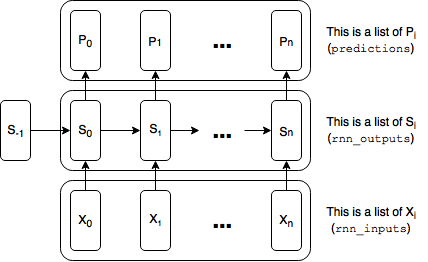
This worked quite well for our toy task, because our longest dependency was 7 steps back and we never really needed to backpropagate errors more than 10 steps. Even with a word-level RNN, using lists will probably be sufficient. See, e.g., my post on Styles of Truncated Backpropagation, where I build a 40-step graph with no problems. But for a character-level model, 40 characters isn’t a whole lot. We might want to capture much longer dependencies. So let’s see what happens when we build a graph that is 200 time steps wide:
def build_basic_rnn_graph_with_list(
    state_size = 100,
    num_classes = vocab_size,
    batch_size = 32,
    num_steps = 200,
    learning_rate = 1e-4):

    reset_graph()

    x = tf.placeholder(tf.int32, [batch_size, num_steps], name='input_placeholder')
    y = tf.placeholder(tf.int32, [batch_size, num_steps], name='labels_placeholder')

    x_one_hot = tf.one_hot(x, num_classes)
    rnn_inputs = [tf.squeeze(i,squeeze_dims=[1]) for i in tf.split(1, num_steps, x_one_hot)]

    cell = tf.nn.rnn_cell.BasicRNNCell(state_size)
    init_state = cell.zero_state(batch_size, tf.float32)
    rnn_outputs, final_state = tf.nn.rnn(cell, rnn_inputs, initial_state=init_state)

    with tf.variable_scope('softmax'):
        W = tf.get_variable('W', [state_size, num_classes])
        b = tf.get_variable('b', [num_classes], initializer=tf.constant_initializer(0.0))
    logits = [tf.matmul(rnn_output, W) + b for rnn_output in rnn_outputs]

    y_as_list = [tf.squeeze(i, squeeze_dims=[1]) for i in tf.split(1, num_steps, y)]

    loss_weights = [tf.ones([batch_size]) for i in range(num_steps)]
    losses = tf.nn.seq2seq.sequence_loss_by_example(logits, y_as_list, loss_weights)
    total_loss = tf.reduce_mean(losses)
    train_step = tf.train.AdamOptimizer(learning_rate).minimize(total_loss)

    return dict(
        x = x,
        y = y,
        init_state = init_state,
        final_state = final_state,
        total_loss = total_loss,
        train_step = train_step
    )
t = time.time()
build_basic_rnn_graph_with_list()
print("It took", time.time() - t, "seconds to build the graph.")It took 5.626644849777222 seconds to build the graph.It took over 5 seconds to build the graph of the most basic RNN model! This could bad… what happens when we move up to a 3-layer LSTM?
Below, we switch out the RNN cell for a Multi-layer LSTM cell. We’ll go over the details of how to do this in the next section.
def build_multilayer_lstm_graph_with_list(
    state_size = 100,
    num_classes = vocab_size,
    batch_size = 32,
    num_steps = 200,
    num_layers = 3,
    learning_rate = 1e-4):

    reset_graph()

    x = tf.placeholder(tf.int32, [batch_size, num_steps], name='input_placeholder')
    y = tf.placeholder(tf.int32, [batch_size, num_steps], name='labels_placeholder')

    embeddings = tf.get_variable('embedding_matrix', [num_classes, state_size])
    rnn_inputs = [tf.squeeze(i) for i in tf.split(1,
                                num_steps, tf.nn.embedding_lookup(embeddings, x))]

    cell = tf.nn.rnn_cell.LSTMCell(state_size, state_is_tuple=True)
    cell = tf.nn.rnn_cell.MultiRNNCell([cell] * num_layers, state_is_tuple=True)
    init_state = cell.zero_state(batch_size, tf.float32)
    rnn_outputs, final_state = tf.nn.rnn(cell, rnn_inputs, initial_state=init_state)

    with tf.variable_scope('softmax'):
        W = tf.get_variable('W', [state_size, num_classes])
        b = tf.get_variable('b', [num_classes], initializer=tf.constant_initializer(0.0))
    logits = [tf.matmul(rnn_output, W) + b for rnn_output in rnn_outputs]

    y_as_list = [tf.squeeze(i, squeeze_dims=[1]) for i in tf.split(1, num_steps, y)]

    loss_weights = [tf.ones([batch_size]) for i in range(num_steps)]
    losses = tf.nn.seq2seq.sequence_loss_by_example(logits, y_as_list, loss_weights)
    total_loss = tf.reduce_mean(losses)
    train_step = tf.train.AdamOptimizer(learning_rate).minimize(total_loss)

    return dict(
        x = x,
        y = y,
        init_state = init_state,
        final_state = final_state,
        total_loss = total_loss,
        train_step = train_step
    )
t = time.time()
build_multilayer_lstm_graph_with_list()
print("It took", time.time() - t, "seconds to build the graph.")It took 25.640846967697144 seconds to build the graph.Yikes, almost 30 seconds.
Now this isn’t that big of an issue for training, because we only need to build the graph once. It could be a big issue, however, if we need to build the graph multiple times at test time.
To get around this long compile time, Tensorflow allows us to create the graph at runtime. Here is a quick demonstration of the difference, using Tensorflow’s dynamic_rnn function:
def build_multilayer_lstm_graph_with_dynamic_rnn(
    state_size = 100,
    num_classes = vocab_size,
    batch_size = 32,
    num_steps = 200,
    num_layers = 3,
    learning_rate = 1e-4):

    reset_graph()

    x = tf.placeholder(tf.int32, [batch_size, num_steps], name='input_placeholder')
    y = tf.placeholder(tf.int32, [batch_size, num_steps], name='labels_placeholder')

    embeddings = tf.get_variable('embedding_matrix', [num_classes, state_size])

    # Note that our inputs are no longer a list, but a tensor of dims batch_size x num_steps x state_size
    rnn_inputs = tf.nn.embedding_lookup(embeddings, x)

    cell = tf.nn.rnn_cell.LSTMCell(state_size, state_is_tuple=True)
    cell = tf.nn.rnn_cell.MultiRNNCell([cell] * num_layers, state_is_tuple=True)
    init_state = cell.zero_state(batch_size, tf.float32)
    rnn_outputs, final_state = tf.nn.dynamic_rnn(cell, rnn_inputs, initial_state=init_state)

    with tf.variable_scope('softmax'):
        W = tf.get_variable('W', [state_size, num_classes])
        b = tf.get_variable('b', [num_classes], initializer=tf.constant_initializer(0.0))

    #reshape rnn_outputs and y so we can get the logits in a single matmul
    rnn_outputs = tf.reshape(rnn_outputs, [-1, state_size])
    y_reshaped = tf.reshape(y, [-1])

    logits = tf.matmul(rnn_outputs, W) + b

    total_loss = tf.reduce_mean(tf.nn.sparse_softmax_cross_entropy_with_logits(logits, y_reshaped))
    train_step = tf.train.AdamOptimizer(learning_rate).minimize(total_loss)

    return dict(
        x = x,
        y = y,
        init_state = init_state,
        final_state = final_state,
        total_loss = total_loss,
        train_step = train_step
    )
t = time.time()
build_multilayer_lstm_graph_with_dynamic_rnn()
print("It took", time.time() - t, "seconds to build the graph.")It took 0.5314393043518066 seconds to build the graph.Much better. One would think that pushing the graph construction to execution time would cause execution of the graph to go slower, but in this case, using dynamic_rnn actually speeds things up:
g = build_multilayer_lstm_graph_with_list()
t = time.time()
train_network(g, 3)
print("It took", time.time() - t, "seconds to train for 3 epochs.")
Average training loss for Epoch 0 : 3.53323210245
Average training loss for Epoch 1 : 3.31435756163
Average training loss for Epoch 2 : 3.21755325109
It took 117.78161263465881 seconds to train for 3 epochs.g = build_multilayer_lstm_graph_with_dynamic_rnn()
t = time.time()
train_network(g, 3)
print("It took", time.time() - t, "seconds to train for 3 epochs.")Average training loss for Epoch 0 : 3.55792756053
Average training loss for Epoch 1 : 3.3225021006
Average training loss for Epoch 2 : 3.28286816745
It took 96.69413661956787 seconds to train for 3 epochs.It’s not a breeze to work through and understand the dynamic_rnn code (which lives here), but we can obtain a similar result ourselves by using tf.scan (dynamic_rnn does not use scan). Scan runs just a tad slower than Tensorflow’s optimized code, but is easier to understand and write yourself.
Scan is a higher-order function that you might be familiar with if you’ve done any programming in OCaml, Haskell or the like. In general, it takes a function (), a sequence () and an initial value () and returns a sequence () according to the rule: . In Tensorflow, scan treats the first dimension of a Tensor as the sequence. Thus, if fed a Tensor of shape [n, m, o] as the sequence, scan would unpack it into a sequence of n-tensors, each with shape [m, o]. You can learn more about Tensorflow’s scan here.
Below, I use scan with an LSTM so as to compare to the dynamic_rnn using Tensorflow above. Because LSTMs store their state in a 2-tuple, and we’re using a 3-layer network, the scan function produces, as final_states below, a 3-tuple (one for each layer) of 2-tuples (one for each LSTM state), each of shape [num_steps, batch_size, state_size]. We need only the last state, which is why we unpack, slice and repack final_states to get final_state below.
Another thing to note is that scan produces rnn_outputs with shape [num_steps, batch_size, state_size], whereas the dynamic_rnn produces rnn_outputs with shape [batch_size, num_steps, state_size] (the first two dimensions are switched). Dynamic_rnn has the flexibility to switch this behavior, using the “time_major” argument. Tf.scan does not have this flexibility, which is why we transpose rnn_inputs and y in the code below.
def build_multilayer_lstm_graph_with_scan(
    state_size = 100,
    num_classes = vocab_size,
    batch_size = 32,
    num_steps = 200,
    num_layers = 3,
    learning_rate = 1e-4):

    reset_graph()

    x = tf.placeholder(tf.int32, [batch_size, num_steps], name='input_placeholder')
    y = tf.placeholder(tf.int32, [batch_size, num_steps], name='labels_placeholder')

    embeddings = tf.get_variable('embedding_matrix', [num_classes, state_size])

    rnn_inputs = tf.nn.embedding_lookup(embeddings, x)

    cell = tf.nn.rnn_cell.LSTMCell(state_size, state_is_tuple=True)
    cell = tf.nn.rnn_cell.MultiRNNCell([cell] * num_layers, state_is_tuple=True)
    init_state = cell.zero_state(batch_size, tf.float32)
    rnn_outputs, final_states = \
        tf.scan(lambda a, x: cell(x, a[1]),
                tf.transpose(rnn_inputs, [1,0,2]),
                initializer=(tf.zeros([batch_size, state_size]), init_state))

    # there may be a better way to do this:
    final_state = tuple([tf.nn.rnn_cell.LSTMStateTuple(
                  tf.squeeze(tf.slice(c, [num_steps-1,0,0], [1, batch_size, state_size])),
                  tf.squeeze(tf.slice(h, [num_steps-1,0,0], [1, batch_size, state_size])))
                       for c, h in final_states])

    with tf.variable_scope('softmax'):
        W = tf.get_variable('W', [state_size, num_classes])
        b = tf.get_variable('b', [num_classes], initializer=tf.constant_initializer(0.0))

    rnn_outputs = tf.reshape(rnn_outputs, [-1, state_size])
    y_reshaped = tf.reshape(tf.transpose(y,[1,0]), [-1])

    logits = tf.matmul(rnn_outputs, W) + b

    total_loss = tf.reduce_mean(tf.nn.sparse_softmax_cross_entropy_with_logits(logits, y_reshaped))
    train_step = tf.train.AdamOptimizer(learning_rate).minimize(total_loss)

    return dict(
        x = x,
        y = y,
        init_state = init_state,
        final_state = final_state,
        total_loss = total_loss,
        train_step = train_step
    )
t = time.time()
g = build_multilayer_lstm_graph_with_scan()
print("It took", time.time() - t, "seconds to build the graph.")
t = time.time()
train_network(g, 3)
print("It took", time.time() - t, "seconds to train for 3 epochs.")It took 0.6475389003753662 seconds to build the graph.
Average training loss for Epoch 0 : 3.55362293501
Average training loss for Epoch 1 : 3.32045680079
Average training loss for Epoch 2 : 3.27433713688
It took 101.60246014595032 seconds to train for 3 epochs.Using scan was only marginally slower than using dynamic_rnn, and gives us the flexibility and understanding to tweak the code if we ever need to (e.g., if for some reason we wanted to create a skip connection from the state at timestep t-2 to timestep t, it would be easy to do with scan).
Upgrading the RNN cell
Above, we seamlessly swapped out the BasicRNNCell we were using for a Multi-layered LSTM cell. This was possible because the RNN cells conform to a general structure: every RNN cell is a function of the current input, , and the prior state, , that outputs a current state, , and a current output, . Thus, in the same way that we can swap out activation functions in a feedforward net (e.g., change the tanh activation to a sigmoid or a relu activation), we can swap out the entire recurrence function (cell) in an RNN.
Note that while for basic RNN cells, the current output equals the current state (), this does not have to be the case. We’ll see how LSTMs and multi-layered RNNs diverge from this below.
Two popular choices for RNN cells are the GRU cell and the LSTM cell. By using gates, GRU and LSTM cells avoid the vanishing gradient problem and allow the network to learn longer-term dependencies. Their internals are quite complicated, and I would refer you to my post Written Memories: Understanding, Deriving and Extending the LSTM for a good starting point to learn about them.
All we have to do to upgrade our vanilla RNN cell is to replace this line:
cell = tf.nn.rnn_cell.BasicRNNCell(state_size)with this for LSTM:
cell = tf.nn.rnn_cell.LSTMCell(state_size)or this for GRU:
cell = tf.nn.rnn_cell.GRUCell(state_size)The LSTM keeps two sets of internal state vectors, (for memory cell or constant error carousel) and (for hidden state). By default, they are concatenated into a single vector, but as of this writing, using the default arguments to LSTMCell will produce a warning message:
WARNING:tensorflow:<tensorflow.python.ops.rnn_cell.LSTMCell object at 0x7faade1708d0>: Using a concatenated state is slower and will soon be deprecated. Use state_is_tuple=True.This error tells us that it’s faster to represent the LSTM state as a tuple of and , rather than as a concatenation of and . You can tack on the argument state_is_tuple=True to have it do that.
By using a tuple for the state, we can also easily replace the base cell with a “MultiRNNCell” for multiple layers. To see why this works, consider that while a single cell:

looks different from a two cells stacked on top of each other:

we can wrap the two cells into a single two-layer cell to make them look and behave as a single cell:

To make this switch, we call tf.nn.rnn_cell.MultiRNNCell, which takes a list of RNNCells as its inputs and wraps them into a single cell:
cell = tf.nn.rnn_cell.MultiRNNCell([tf.nn.rnn_cell.BasicRNNCell(state_size)] * num_layers)Note that if you are wrapping an LSTMCell that uses state_is_tuple=True, you should pass this same argument to the MultiRNNCell as well.
Writing a custom RNN cell
It’s almost too easy to use the standard GRU or LSTM cells, so let’s define our own RNN cell. Here’s a random idea that may or may not work: starting with a GRU cell, instead of taking a single transformation of its input, we enable it to take a weighted average of multiple transformations of its input. That is, using the notation from Cho et al. (2014), instead of using in our candidate state, , we use a weighted average of for some n. In other words, we will replace with for some weights that sum to 1. The vector of weights, , will be calculated as . The idea is that we might benefit from treat the input differently in different scenarios (e.g., we may want to treat verbs differently than nouns).
To write the custom cell, we need to extend tf.nn.rnn_cell.RNNCell. Specifically, we need to fill in 3 abstract methods and write an __init__ method (take a look at the Tensorflow code here). First, let’s start with a GRU cell, adapted from Tensorflow’s implementation:
class GRUCell(tf.nn.rnn_cell.RNNCell):
    """Gated Recurrent Unit cell (cf. http://arxiv.org/abs/1406.1078)."""

    def __init__(self, num_units):
        self._num_units = num_units

    @property
    def state_size(self):
        return self._num_units

    @property
    def output_size(self):
        return self._num_units

    def __call__(self, inputs, state, scope=None):
        with tf.variable_scope(scope or type(self).__name__):  # "GRUCell"
            with tf.variable_scope("Gates"):  # Reset gate and update gate.
                # We start with bias of 1.0 to not reset and not update.
                ru = tf.nn.rnn_cell._linear([inputs, state],
                                        2 * self._num_units, True, 1.0)
                ru = tf.nn.sigmoid(ru)
                r, u = tf.split(1, 2, ru)
            with tf.variable_scope("Candidate"):
                c = tf.nn.tanh(tf.nn.rnn_cell._linear([inputs, r * state],
                                             self._num_units, True))
            new_h = u * state + (1 - u) * c
        return new_h, new_h
We modify the __init__ method to take a parameter at initialization, which will determine the number of transformation matrices it will create:
def __init__(self, num_units, num_weights):
    self._num_units = num_units
    self._num_weights = num_weights
Then, we modify the Candidate variable scope of the __call__ method to do a weighted average as shown below (note that all of the matrices are created as a single variable and then split into multiple tensors):
class CustomCell(tf.nn.rnn_cell.RNNCell):
    """Gated Recurrent Unit cell (cf. http://arxiv.org/abs/1406.1078)."""

    def __init__(self, num_units, num_weights):
        self._num_units = num_units
        self._num_weights = num_weights

    @property
    def state_size(self):
        return self._num_units

    @property
    def output_size(self):
        return self._num_units

    def __call__(self, inputs, state, scope=None):
        with tf.variable_scope(scope or type(self).__name__):  # "GRUCell"
            with tf.variable_scope("Gates"):  # Reset gate and update gate.
                # We start with bias of 1.0 to not reset and not update.
                ru = tf.nn.rnn_cell._linear([inputs, state],
                                        2 * self._num_units, True, 1.0)
                ru = tf.nn.sigmoid(ru)
                r, u = tf.split(1, 2, ru)
            with tf.variable_scope("Candidate"):
                lambdas = tf.nn.rnn_cell._linear([inputs, state], self._num_weights, True)
                lambdas = tf.split(1, self._num_weights, tf.nn.softmax(lambdas))

                Ws = tf.get_variable("Ws",
                        shape = [self._num_weights, inputs.get_shape()[1], self._num_units])
                Ws = [tf.squeeze(i) for i in tf.split(0, self._num_weights, Ws)]

                candidate_inputs = []

                for idx, W in enumerate(Ws):
                    candidate_inputs.append(tf.matmul(inputs, W) * lambdas[idx])

                Wx = tf.add_n(candidate_inputs)

                c = tf.nn.tanh(Wx + tf.nn.rnn_cell._linear([r * state],
                                            self._num_units, True, scope="second"))
            new_h = u * state + (1 - u) * c
        return new_h, new_h
Let’s see how the custom cell stacks up to a regular GRU cell (using num_steps = 30, since this performs much better than num_steps = 200 after 5 epochs – can you see why that might happen?):
def build_multilayer_graph_with_custom_cell(
    cell_type = None,
    num_weights_for_custom_cell = 5,
    state_size = 100,
    num_classes = vocab_size,
    batch_size = 32,
    num_steps = 200,
    num_layers = 3,
    learning_rate = 1e-4):

    reset_graph()

    x = tf.placeholder(tf.int32, [batch_size, num_steps], name='input_placeholder')
    y = tf.placeholder(tf.int32, [batch_size, num_steps], name='labels_placeholder')

    embeddings = tf.get_variable('embedding_matrix', [num_classes, state_size])

    rnn_inputs = tf.nn.embedding_lookup(embeddings, x)

    if cell_type == 'Custom':
        cell = CustomCell(state_size, num_weights_for_custom_cell)
    elif cell_type == 'GRU':
        cell = tf.nn.rnn_cell.GRUCell(state_size)
    elif cell_type == 'LSTM':
        cell = tf.nn.rnn_cell.LSTMCell(state_size, state_is_tuple=True)
    else:
        cell = tf.nn.rnn_cell.BasicRNNCell(state_size)

    if cell_type == 'LSTM':
        cell = tf.nn.rnn_cell.MultiRNNCell([cell] * num_layers, state_is_tuple=True)
    else:
        cell = tf.nn.rnn_cell.MultiRNNCell([cell] * num_layers)

    init_state = cell.zero_state(batch_size, tf.float32)
    rnn_outputs, final_state = tf.nn.dynamic_rnn(cell, rnn_inputs, initial_state=init_state)

    with tf.variable_scope('softmax'):
        W = tf.get_variable('W', [state_size, num_classes])
        b = tf.get_variable('b', [num_classes], initializer=tf.constant_initializer(0.0))

    #reshape rnn_outputs and y
    rnn_outputs = tf.reshape(rnn_outputs, [-1, state_size])
    y_reshaped = tf.reshape(y, [-1])

    logits = tf.matmul(rnn_outputs, W) + b

    total_loss = tf.reduce_mean(tf.nn.sparse_softmax_cross_entropy_with_logits(logits, y_reshaped))
    train_step = tf.train.AdamOptimizer(learning_rate).minimize(total_loss)

    return dict(
        x = x,
        y = y,
        init_state = init_state,
        final_state = final_state,
        total_loss = total_loss,
        train_step = train_step
    )
g = build_multilayer_graph_with_custom_cell(cell_type='GRU', num_steps=30)
t = time.time()
train_network(g, 5, num_steps=30)
print("It took", time.time() - t, "seconds to train for 5 epochs.")Average training loss for Epoch 0 : 2.92919953048
Average training loss for Epoch 1 : 2.35888109404
Average training loss for Epoch 2 : 2.21945820894
Average training loss for Epoch 3 : 2.12258511006
Average training loss for Epoch 4 : 2.05038544733
It took 284.6971204280853 seconds to train for 5 epochs.g = build_multilayer_graph_with_custom_cell(cell_type='Custom', num_steps=30)
t = time.time()
train_network(g, 5, num_steps=30)
print("It took", time.time() - t, "seconds to train for 5 epochs.")Average training loss for Epoch 0 : 3.04418995892
Average training loss for Epoch 1 : 2.5172702761
Average training loss for Epoch 2 : 2.37068433601
Average training loss for Epoch 3 : 2.27533404217
Average training loss for Epoch 4 : 2.20167231745
It took 537.6112766265869 seconds to train for 5 epochs.So much for that idea. Our custom cell took almost twice as long to train and seems to perform worse than a standard GRU cell.
Adding Dropout
Adding features like dropout to the network is easy: we figure out where they belong and drop them in.
Dropout belongs in between layers, not on the state or in intra-cell connections. See Zaremba et al. (2015), Recurrent Neural Network Regularization (“The main idea is to apply the dropout operator only to the non-recurrent connections.”)
Thus, to apply dropout, we need to wrap the input and/or output of each cell. In our RNN implementation using list, we might do something like this:
rnn_inputs = [tf.nn.dropout(rnn_input, keep_prob) for rnn_input in rnn_inputs]
rnn_outputs = [tf.nn.dropout(rnn_output, keep_prob) for nn_output in rnn_outputs]
In our dynamic_rnn or scan implementations, we might apply dropout directly to the rnn_inputs or rnn_outputs:
rnn_inputs = tf.nn.dropout(rnn_inputd, keep_prob)
rnn_outputs = tf.nn.dropout(rnn_outputd, keep_prob)
But what happens when we use MultiRNNCell? How can we have dropout in between layers like in Zaremba et al. (2015)? The answer is to wrap our base RNN cell with dropout, thereby including it as part of the base cell, similar to how we wrapped our three RNN cells into a single MultiRNNCell above. Tensorflow allows us to do this without writing a new RNNCell by using tf.nn.rnn_cell.DropoutWrapper:
cell = tf.nn.rnn_cell.LSTMCell(state_size, state_is_tuple=True)
cell = tf.nn.rnn_cell.DropoutWrapper(cell, input_keep_prob=input_dropout, output_keep_prob=output_dropout)
cell = tf.nn.rnn_cell.MultiRNNCell([cell] * num_layers, state_is_tuple=True)
Note that if we wrap a base cell with dropout and then use it to build a MultiRNNCell, both input dropout and output dropout will be applied between layers (so if both are, say, 0.9, the dropout in between layers will be 0.9 * 0.9 = 0.81). If we want equal dropout on all inputs and outputs of a multi-layered RNN, we can use only output or input dropout on the base cell, and then wrap the entire MultiRNNCell with the input or output dropout like so:
cell = tf.nn.rnn_cell.LSTMCell(state_size, state_is_tuple=True)
cell = tf.nn.rnn_cell.DropoutWrapper(cell, input_keep_prob=global_dropout)
cell = tf.nn.rnn_cell.MultiRNNCell([cell] * num_layers, state_is_tuple=True)
cell = tf.nn.rnn_cell.DropoutWrapper(cell, output_keep_prob=global_dropout)
Layer normalization
Layer normalization is a feature that was published just a few days ago by Lei Ba et al. (2016), which we can use to improve our RNN. It was inspired by batch normalization, which you can read about and learn how to implement in my post here. Batch normalization (for feed-forward and convolutional neural networks) and layer normalization (for recurrent neural networks) generally improve training time and achieve better overall performance. In this section, we’ll apply what we’ve learned in this post to implement layer normalization in Tensorflow.
Layer normalization is applied as follows: the initial layer normalization function is applied individually to each training example so as to normalize the output vector of a linear transformation to have a mean of 0 and a variance of 1. In math: for some vector and some small value of for numerical stability. For some the same reasons we add scale and shift parameters to the initial batch normalization transform (see my batch normalization post for details), we add scale, , and shift, , parameters here as well, so that the final layer normalization function is:
Note that is point-wise multiplication.
To add layer normalization to our network, we first write a function that will layer normalization a 2D tensor along its second dimension:
def ln(tensor, scope = None, epsilon = 1e-5):
    """ Layer normalizes a 2D tensor along its second axis """
    assert(len(tensor.get_shape()) == 2)
    m, v = tf.nn.moments(tensor, [1], keep_dims=True)
    if not isinstance(scope, str):
        scope = ''
    with tf.variable_scope(scope + 'layer_norm'):
        scale = tf.get_variable('scale',
                                shape=[tensor.get_shape()[1]],
                                initializer=tf.constant_initializer(1))
        shift = tf.get_variable('shift',
                                shape=[tensor.get_shape()[1]],
                                initializer=tf.constant_initializer(0))
    LN_initial = (tensor - m) / tf.sqrt(v + epsilon)

    return LN_initial * scale + shift
Let’s apply it our layer normalization function as it was applied by Lei Ba et al. (2016) to LSTMs (in their experiments “Teaching machines to read and comprehend” and “Handwriting sequence generation”). Lei Ba et al. apply layer normalization to the output of each gate inside the LSTM cell, which means that we get to take a second shot at writing a new type of RNN cell. We’ll start with Tensorflow’s official code, located here, and modify it accordingly:
class LayerNormalizedLSTMCell(tf.nn.rnn_cell.RNNCell):
    """
    Adapted from TF's BasicLSTMCell to use Layer Normalization.
    Note that state_is_tuple is always True.
    """

    def __init__(self, num_units, forget_bias=1.0, activation=tf.nn.tanh):
        self._num_units = num_units
        self._forget_bias = forget_bias
        self._activation = activation

    @property
    def state_size(self):
        return tf.nn.rnn_cell.LSTMStateTuple(self._num_units, self._num_units)

    @property
    def output_size(self):
        return self._num_units

    def __call__(self, inputs, state, scope=None):
        """Long short-term memory cell (LSTM)."""
        with tf.variable_scope(scope or type(self).__name__):
            c, h = state

            # change bias argument to False since LN will add bias via shift
            concat = tf.nn.rnn_cell._linear([inputs, h], 4 * self._num_units, False)

            i, j, f, o = tf.split(1, 4, concat)

            # add layer normalization to each gate
            i = ln(i, scope = 'i/')
            j = ln(j, scope = 'j/')
            f = ln(f, scope = 'f/')
            o = ln(o, scope = 'o/')

            new_c = (c * tf.nn.sigmoid(f + self._forget_bias) + tf.nn.sigmoid(i) *
                   self._activation(j))

            # add layer_normalization in calculation of new hidden state
            new_h = self._activation(ln(new_c, scope = 'new_h/')) * tf.nn.sigmoid(o)
            new_state = tf.nn.rnn_cell.LSTMStateTuple(new_c, new_h)

            return new_h, new_state
And that’s it! Let’s try this out.
Final model
At this point, we’ve covered all of the graph modifications we planned to cover, so here is our final model, which allows for dropout and layer normalized LSTM cells:
def build_graph(
    cell_type = None,
    num_weights_for_custom_cell = 5,
    state_size = 100,
    num_classes = vocab_size,
    batch_size = 32,
    num_steps = 200,
    num_layers = 3,
    build_with_dropout=False,
    learning_rate = 1e-4):

    reset_graph()

    x = tf.placeholder(tf.int32, [batch_size, num_steps], name='input_placeholder')
    y = tf.placeholder(tf.int32, [batch_size, num_steps], name='labels_placeholder')

    dropout = tf.constant(1.0)

    embeddings = tf.get_variable('embedding_matrix', [num_classes, state_size])

    rnn_inputs = tf.nn.embedding_lookup(embeddings, x)

    if cell_type == 'Custom':
        cell = CustomCell(state_size, num_weights_for_custom_cell)
    elif cell_type == 'GRU':
        cell = tf.nn.rnn_cell.GRUCell(state_size)
    elif cell_type == 'LSTM':
        cell = tf.nn.rnn_cell.LSTMCell(state_size, state_is_tuple=True)
    elif cell_type == 'LN_LSTM':
        cell = LayerNormalizedLSTMCell(state_size)
    else:
        cell = tf.nn.rnn_cell.BasicRNNCell(state_size)

    if build_with_dropout:
        cell = tf.nn.rnn_cell.DropoutWrapper(cell, input_keep_prob=dropout)

    if cell_type == 'LSTM' or cell_type == 'LN_LSTM':
        cell = tf.nn.rnn_cell.MultiRNNCell([cell] * num_layers, state_is_tuple=True)
    else:
        cell = tf.nn.rnn_cell.MultiRNNCell([cell] * num_layers)

    if build_with_dropout:
        cell = tf.nn.rnn_cell.DropoutWrapper(cell, output_keep_prob=dropout)

    init_state = cell.zero_state(batch_size, tf.float32)
    rnn_outputs, final_state = tf.nn.dynamic_rnn(cell, rnn_inputs, initial_state=init_state)

    with tf.variable_scope('softmax'):
        W = tf.get_variable('W', [state_size, num_classes])
        b = tf.get_variable('b', [num_classes], initializer=tf.constant_initializer(0.0))

    #reshape rnn_outputs and y
    rnn_outputs = tf.reshape(rnn_outputs, [-1, state_size])
    y_reshaped = tf.reshape(y, [-1])

    logits = tf.matmul(rnn_outputs, W) + b

    predictions = tf.nn.softmax(logits)

    total_loss = tf.reduce_mean(tf.nn.sparse_softmax_cross_entropy_with_logits(logits, y_reshaped))
    train_step = tf.train.AdamOptimizer(learning_rate).minimize(total_loss)

    return dict(
        x = x,
        y = y,
        init_state = init_state,
        final_state = final_state,
        total_loss = total_loss,
        train_step = train_step,
        preds = predictions,
        saver = tf.train.Saver()
    )
Let’s compare the GRU, LSTM and LN_LSTM after training each for 20 epochs using 80 step sequences.
g = build_graph(cell_type='GRU', num_steps=80)
t = time.time()
losses = train_network(g, 20, num_steps=80, save="saves/GRU_20_epochs")
print("It took", time.time() - t, "seconds to train for 20 epochs.")
print("The average loss on the final epoch was:", losses[-1])
It took 1051.6652357578278 seconds to train for 20 epochs.
The average loss on the final epoch was: 1.75318197903g = build_graph(cell_type='LSTM', num_steps=80)
t = time.time()
losses = train_network(g, 20, num_steps=80, save="saves/LSTM_20_epochs")
print("It took", time.time() - t, "seconds to train for 20 epochs.")
print("The average loss on the final epoch was:", losses[-1])It took 614.4890048503876 seconds to train for 20 epochs.
The average loss on the final epoch was: 2.02813237837g = build_graph(cell_type='LN_LSTM', num_steps=80)
t = time.time()
losses = train_network(g, 20, num_steps=80, save="saves/LN_LSTM_20_epochs")
print("It took", time.time() - t, "seconds to train for 20 epochs.")
print("The average loss on the final epoch was:", losses[-1])It took 3867.550405740738 seconds to train for 20 epochs.
The average loss on the final epoch was: 1.71850851623It looks like the layer normalized LSTM just managed to edge out the GRU in the last few epochs, though the increase in training time hardly seems worth it (perhaps my implementation could be improved?). It would be interesting to see how they would perform on a validation or test set and also to try out a layer normalized GRU. For now, let’s use the GRU to generate some text.
Generating text
To generate text, were going to rebuild the graph so as to accept a single character at a time and restore our saved model. We’ll give the network a single character prompt, grab its predicted probability distribution for the next character, use that distribution to pick the next character, and repeat. When picking the next character, our generate_characters function can be set to use the whole probability distribution (default), or be forced to pick one of the top n most likely characters in the distribution. The latter option should obtain more English-like results.
def generate_characters(g, checkpoint, num_chars, prompt='A', pick_top_chars=None):
    """ Accepts a current character, initial state"""

    with tf.Session() as sess:
        sess.run(tf.initialize_all_variables())
        g['saver'].restore(sess, checkpoint)

        state = None
        current_char = vocab_to_idx[prompt]
        chars = [current_char]

        for i in range(num_chars):
            if state is not None:
                feed_dict={g['x']: [[current_char]], g['init_state']: state}
            else:
                feed_dict={g['x']: [[current_char]]}

            preds, state = sess.run([g['preds'],g['final_state']], feed_dict)

            if pick_top_chars is not None:
                p = np.squeeze(preds)
                p[np.argsort(p)[:-pick_top_chars]] = 0
                p = p / np.sum(p)
                current_char = np.random.choice(vocab_size, 1, p=p)[0]
            else:
                current_char = np.random.choice(vocab_size, 1, p=np.squeeze(preds))[0]

            chars.append(current_char)

    chars = map(lambda x: idx_to_vocab[x], chars)
    print("".join(chars))
    return("".join(chars))
g = build_graph(cell_type='LN_LSTM', num_steps=1, batch_size=1)
generate_characters(g, "saves/LN_LSTM_20_epochs", 750, prompt='A', pick_top_chars=5)ATOOOS
UIEAOUYOUZZZZZZUZAAAYAYf n fsflflrurctuateot t ta's a wtutss ESGNANO:
Whith then, a do makes and them and to sees,
I wark on this ance may string take thou honon
To sorriccorn of the bairer, whither, all
I'd see if yiust the would a peid.
LARYNGLe:
To would she troust they fould.
PENMES:
Thou she so the havin to my shald woust of
As tale we they all my forder have
As to say heant thy wansing thag and
Whis it thee shath his breact, I be and might, she
Tirs you desarvishensed and see thee: shall,
What he hath with that is all time,
And sen the have would be sectiens, way thee,
They are there to man shall with me to the mon,
And mere fear would be the balte, as time an at
And the say oun touth, thy way womers thee.You can see that this network has learned something. It’s definitely not random, though there is a bit of a warm up at the beginning (the state starts at 0). I was expecting something a bit better, however, given Karpathy’s Shakespeare results. His model used more data, a state_size of 512, and was trained quite a bit longer than this one. Let’s see if we can match that. I couldn’t find a suitable premade dataset, so I had to make one myself: I concatenated the scripts from the Star Wars movies, the Star Trek movies, Tarantino and the Matrix. The final file size is 3.3MB, which is a bit smaller than the full works of William Shakespeare. Let’s load these up and try this again, with a larger state size:
"""
Load new data
"""

file_url = 'https://gist.githubusercontent.com/spitis/59bfafe6966bfe60cc206ffbb760269f/'+\
'raw/030a08754aada17cef14eed6fac7797cda830fe8/variousscripts.txt'
file_name = 'variousscripts.txt'
if not os.path.exists(file_name):
    urllib.request.urlretrieve(file_url, file_name)

with open(file_name,'r') as f:
    raw_data = f.read()
    print("Data length:", len(raw_data))

vocab = set(raw_data)
vocab_size = len(vocab)
idx_to_vocab = dict(enumerate(vocab))
vocab_to_idx = dict(zip(idx_to_vocab.values(), idx_to_vocab.keys()))

data = [vocab_to_idx[c] for c in raw_data]
del raw_data
Data length: 3299132g = build_graph(cell_type='GRU',
num_steps=80,
state_size = 512,
batch_size = 50,
num_classes=vocab_size,
learning_rate=5e-4)
t = time.time()
losses = train_network(g, 30, num_steps=80, batch_size = 50, save="saves/GRU_30_epochs_variousscripts")
print("It took", time.time() - t, "seconds to train for 30 epochs.")
print("The average loss on the final epoch was:", losses[-1])It took 4877.8002140522 seconds to train for 30 epochs.
The average loss on the final epoch was: 0.726858645461g = build_graph(cell_type='GRU', num_steps=1, batch_size=1, num_classes=vocab_size, state_size = 512)
generate_characters(g, "saves/GRU_30_epochs_variousscripts", 750, prompt='D', pick_top_chars=5)DENT'SUEENCK
Bartholomew of the TIE FIGHTERS are stunned. There is a crowd and armored
switcheroos.
PICARD
(continuing)
Couns two dim is tired. In order to the sentence...
The sub bottle appears on the screen into a small shuttle shift of the
ceiling. The DAMBA FETT splash fires and matches them into the top, transmit to stable high above upon their statels,
falling from an alien shaft.
ANAKIN and OBI-WAN stand next to OBI-WAN down the control plate of smoke at the TIE fighter. They stare at the centre of the station loose into a comlink cover -- comes up to the General, the GENERAL HUNTAN AND FINNFURMBARD from the PICADOR to a beautiful Podracisly.
ENGINEER
Naboo from an army seventy medical
security team area re-weilergular.
EXT.Not sure these are that much better than before, but it’s sort of readable?
Conclusion
In this post, we used a character sequence generation task to learn how to use Tensorflow’s scan and dynamic_rnn functions, how to use advanced RNN cells and stack multiple RNNs, and how to add features to our RNN like dropout and layer normalization. In the next post, we will use a machine translation task to look at handling variable length sequences and building RNN encoders and decoders.