This post is a preliminary note on the “complexity” of neural networks. It’s a topic that has not gotten much attention in the literature, yet is of central importance to our general understanding of neural networks. In this post I discuss complexity and generalization in broad terms, and make the argument that network structure (including parameter counts), the training methodology, and the regularizers used, though each different in concept, all contribute to this notion of neural network “complexity”.
Model complexity and selection
In designing neural networks there is an inevitable trade-off between model complexity and generalization performance. On one hand, we want the model to be expressive and have the ability to model highly complex non-linear relationships. On the other hand, the more expressive the model, the more capable it is of memorizing the training data. This is the problem of model selection and it is closely related to the “complexity” of the model: pick a model that is too simple and it will “underfit” the data, but pick a model that is too complex and it will “overfit” the data.
There is no consistent analytical definition of complexity, but one reasonable way of to think about it is the effective number of distinct hypotheses the model could potentially represent after training; i.e., the effective number of patterns that the model is capable of describing. See, e.g., Abu-Mostafa eta al. or Myung et al. (2000).
When it comes to neural networks, this notion of complexity and the problem of model selection are delicate subjects. Whereas certain analytical criteria exist for balancing complexity and generalization in traditional statistical models, these criteria have not been extended in any compelling, generally applicable way to the analysis neural networks.1 As a result, the primary approach for neural network model selection has not been analytical, but rather empirical: cross-validation.
This is unfortunate because it is difficult to compare neural network architectures using only empirical tests. One reason for this is that the effects of different architectural features and hyperparameters on complexity are not necessarily independent, which means that the size of the search grows exponentially in the number of features or hyperparameters (including, e.g., the choice of regularizers). Furthermore, these effects are not necessarily independent of the dataset (e.g., a feature that is ineffective on a small dataset may be very effective on a large one), and so results may not generalize across tasks. As a single state of the art model can take hours, days or even weeks to train on modern hardware, this spells bad news for finding the “best” model. Cf., e.g., Chung et al. (2014) (conducts an empirical comparison of the GRU and LSTM and is unable to determine whether one architecture is superior to the other).
This difficulty is not restricted to comparing entire architectures: the fact that adding or removing a feature changes the model complexity makes it difficult to evaluate the efficacy of that single feature. This generally affects the strength of results favoring proposed features in the literature.
But not all hope is lost. In some cases, we can put forth theoretical grounds for the superiority of one architecture over another. See, e.g., my post on Written Memories, which argues that the proposed pseudo LSTM is objectively better than the basic LSTM. In other cases, an architecture or feature overwhelmingly outperforms the competition in a wide range of configurations. In these cases, we can assume the position that one architecture is superior than another, while keeping in the back of our minds the possibility that our conclusion may not generalize to all cases. Sometimes (and ideally), a proposed feature has both strong theoretical grounds and undeniably empirical performance. See, e.g., Ioffe and Szegedy (2015), which introduced batch normalization for feedforward neural networks.
Yet in most cases, we are stuck with many alternatives and little guidance as to how to choose between them, or as to whether such choices even matter. If we had some broadly applicable and theoretically grounded measure of model complexity at our disposal, it would be incredibly useful for making such determinations. I am planning a follow-up post to explore this problem in more detail. For this preliminary note, however, I want to make a few comments on the factors that contribute to model complexity, which include the network structure, the training methodology and the regularization methods used.
Network structure
It’s quite common for authors to use the “number of parameters” as a proxy for model complexity to support the inference that one architecture is better than another (with fewer parameters being better). See e.g., Zilly et al. (2016) (“[Our model] outperforms [the competing model] using less than half the parameters…”), Kim et al. (2015) (“[Our model] is on par with the existing state-of-the-art despite having 60% fewer parameters.”), and Wu et al. (2016)(“… the number of parameters [is] largely reduced, which makes our model more practical for large scale problems, while avoiding overfitting.” (emphasis added)), among many others. I sympathize with the approach, if only because there exists no established criteria for measuring parametric complexity of neural networks, but using simple parameter counts for this purpose is misleading.2
In particular, different models with the same number of parameters may have quite different complexities as result of the model’s functional form. This is true for all models, not just neural networks. As a trivial example, consider that the double biases in the model are really one parameter masquerading as two. See Myung et al. (2000) for a non-trivial example and a more detailed discussion of the “geometric complexity”. As compared to traditional statistical models, however, neural networks are particularly succeptible to this kind of structural complexity; the number of hidden layers, the connectivity between them, and the activation functions used are just a few examples of structural features that impact network complexity. That said, if the network structure of two models is similar (e.g., same number of layers and same activation functions), the complexity of the model will generally be a monotonically increasing function of the number of parameters.
Training method
It might be surprising that the training method (e.g., the combination of initialization method, loss function and optimization algorithm) can be viewed as a factor in model complexity. To see this, consider that the complexity of a model can be interpretted as the effective number of patterns the model can represent after training, but that even if some choice of parameters could represent pattern A, pattern A may not be reachable gradient descent (or, more likely, pattern A could be very difficult to reach relative to pattern B). Here is an illustration:
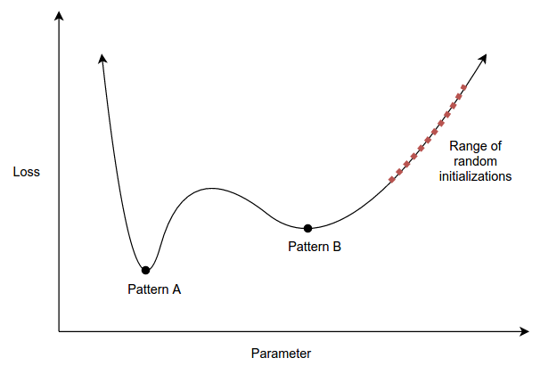
Note that this illustration is oversimplified, in that we would have to consider the “reachableness” of pattern A under all potential datasets, not just this one dataset.
This is an interesting perspective that has a slightly different flavor than criteria such as Rissanen’s minimum description length. Taking this broad view of complexity, we see that the learning rate, which is the first hyperparameter we tune when training neural networks, directly impacts the model’s complexity. E.g., a high learning rate will bias our model away from local minima that are located in narrow valleys. This same argument applies to batch size and truncated backpropagation steps.
Regularization
Finally, somewhere in between structural features and the training method lie regularizers. Consider that dropout can be viewed as a modification to the training method (since the model’s architecture is unchanged at test time) or as an ensemble method (see, e.g., Baldi and Sadowski (2013)). Similarly, weight decay might be viewed as a direct modification to the loss function that modifies the training method, or as a structural feature. To see how weight decay can be interpretted as a structural feature, compare it to a hard “cap” on the parameters, say a restriction to the interval [-0.5, 0.5]. This is a structural change that impacts the number of representable hypotheses, but the function of weight decay is very similar, only that it serves as a soft cap.
Future Work
This topic has been on my mind recently as I wrestle with the question of how to justify an argument that one architecture is better than another. I’m currently working toward a couple preliminary ideas for an analytical approach to neural network complexity, which I will write about in case they pan out. In the meantime, if you are aware of any research in this area, I would greatly appreciate if you could share it in the comments!
There have, however, been specific applications of these analytical criteria. See, e.g., Hinton and van Camp (1993), which shows how weight decay and weight noise can be justified using the minimum description length (MDL) criteria.↩
It’s true that models with fewer parameters will be smaller in size (memory footprint / space), which could be advantageous for large models. The intent of pointing out a lower parameter count, however, is usually to signify that the model is less complex and therefore less prone to overfitting.↩