In this post, I introduce and discuss binary stochastic neurons, implement trainable binary stochastic neurons in Tensorflow, and conduct several simple experiments on the MNIST dataset to get a feel for their behavior. Binary stochastic neurons offer two advantages over real-valued neurons: they can act as a regularizer and they enable conditional computation by enabling a network to make yes/no decisions. Conditional computation opens the door to new and exciting neural network architectures, such as the choice of experts architecture and heirarchical multiscale neural networks, which I plan to discuss in future posts.
The binary stochastic neuron
A binary stochastic neuron is a neuron with a noisy output: some proportion p of the time it outputs 1, otherwise 0. An easy way to turn a real-valued input, a, into this proportion, p, is to set p=sigm(a), where sigm is the logistic sigmoid, sigm(x)=11+exp(−x). Thus, we define the binary stochastic neuron, BSN, as:
BSN(a)=1z < sigm(a)
where 1x is the indicator function on the truth value of x and z∼U[0,1].
Advantages of the binary stochastic neuron
A binary stochastic neuron is a noisy modification of the logistic sigmoid: instead of outputting p, it outputs 1 with probability p and 0 otherwise. Noise generally serves as a regularizer (see, e.g., Srivastava et al. (2014) and Neelakantan et al. (2015)), and so we might expect the same from binary stochastic neurons as compared to the logistic neurons. Indeed, this is the claimed “unpublished result” from the end of Hinton et al.’s Coursera Lecture 9c, which I demonstrate empirically in this post.
Further, by enabling networks to make binary decisions, the binary stochastic neuron allows for conditional computation. This opens the door to some interesting new architectures. For example, instead of a mixture of experts architecture, which weights the outputs of several “expert” sub-networks and requires that all subnetworks be computed, we could use a choice of experts architecture, which conditionally uses expert sub-networks as needed. This architecture is implicitly proposed in Bengio et al. (2013), wherein the experiments use a choice of expert units architecture (i.e., a gated architecture where gates must be 1 or 0). Another example, proposed in Bengio et al. (2013) and implemented by Chung et al. (2016), is the Heirarchical Multiscale Recurrent Neural Network (HM-RNN) architecture, which achieves great results on language modelling tasks.
Training the binary stochastic neuron
For any single trial, the binary stochastic neuron generally has a derivative of 0 and cannot be trained by simple backpropagation. To see this, consider that if z≠sigm(a) in the BSN function above, there exists a neighborhood around a such that the output of BSN(a) is unchanged (i.e., the derivative is 0). We get around this by estimating the derivative with respect to the expected loss, rather than calculating the derivative with respect to the outcome of a single trial. We can only estimate this derivative, because in any given trial, we only see the loss value with respect to the given noise – we don’t know what the loss would have been given another level of noise. We call a method that provides such an estimate an “estimator”. An estimator is unbiased if the expectation of its estimate equals the expectation of the derivative it is estimating; otherwise, it is biased.
In this post we implement the two estimators discussed in Bengio et al. (2013):
The REINFORCE estimator, which is an unbiased estimator and a special case of the REINFORCE algorithm discussed in Williams (1992).
The REINFORCE estimator estimates the expectation of ∂L∂a as (BSN(a)−sigm(a))(L−c), where c is a constant. Bengio et al. (2013) proves that:
E[(BSN(a)−sigm(a))(L−c)]=E[∂L∂a].
Bengio et al. (2013) further shows that to minimize the variance of the estimation, we choose:
c=ˉL=E[BSN(a)−sigm(a))2L]E[BSN(a)−sigm(a))2]
which we can practically implement by keeping track of the numerator and denominator as a moving average. Interestingly, the REINFORCE estimator does not require any backpropagated loss gradient–it operates directly on the loss of the network.
The straight through (ST) estimator, which is a biased estimator that was first proposed by Hinton et al.’s Coursera Lecture 9c.
The ST estimator simply replaces the derivative factor used during backpropagation, dBSN(a)da=0, with the identity function dBSN(a)da=1.1 A variant of the ST estimator replaces the derivative factor with dBSN(a)da=dsigm(a)da. Whereas Bengio et al. (2013) found that the former is more effective, the latter variant was successfully used in Chung et al. (2016) in combination with the slope-annealing trick and deterministic binary neurons (which we will see perform very similarly to, if not better than, stochastic binary neurons when used with slope-annealing). The slope-anealing trick modifies BSN(a) by first multiplying the input a by a slope m as follows:
BSNSL(m)(a)=1z<sigm(ma).
Then, we increase the slope as training progresses and use dBSNSL(m)(a)da=dsigm(ma)da when computing the gradient. The idea behind this is that as the slope increases, the logistic sigmoid approaches a step function, so that it’s derivative approaches the true derivative. All three variants are tested in this post.
Implementing the binary stochastic neuron in Tensorflow
The tricky part of implementing a binary stochastic neuron in Tensorflow is not the forward computation, but the implementation of the REINFORCE and straight through estimators. Each requires replacing the gradient of one or more Tensorflow operations. The official approach to this is to write a new op in C++, which seems wholly unnecessary. There are, however, two workable unofficial approaches, one of which is a trick credited to Sergey Ioffe, and another that uses gradient_override_map, an experimental feature of Tensorflow that is documented here. We will use gradient_override_map, which works well for our purposes.
Imports and Utility Functions
import numpy as np
import tensorflow as tf
from tensorflow.examples.tutorials.mnist import input_data
import matplotlib.pyplot as plt
%matplotlib inline
mnist = input_data.read_data_sets('MNIST_data', one_hot=True)
from tensorflow.python.framework import ops
from enum import Enum
import seaborn as sns
sns.set(color_codes=True)

def reset_graph():
    if 'sess' in globals() and sess:
        sess.close()
    tf.reset_default_graph()

def layer_linear(inputs, shape, scope='linear_layer'):
    with tf.variable_scope(scope):
        w = tf.get_variable('w',shape)
        b = tf.get_variable('b',shape[-1:])
    return tf.matmul(inputs,w) + b

def layer_softmax(inputs, shape, scope='softmax_layer'):
    with tf.variable_scope(scope):
        w = tf.get_variable('w',shape)
        b = tf.get_variable('b',shape[-1:])
    return tf.nn.softmax(tf.matmul(inputs,w) + b)

def accuracy(y, pred):
    correct = tf.equal(tf.argmax(y,1), tf.argmax(pred,1))
    return tf.reduce_mean(tf.cast(correct, tf.float32))

def plot_n(data_and_labels, lower_y = 0., title="Learning Curves"):
    fig, ax = plt.subplots()
    for data, label in data_and_labels:
        ax.plot(range(0,len(data)*100,100),data, label=label)
    ax.set_xlabel('Training steps')
    ax.set_ylabel('Accuracy')
    ax.set_ylim([lower_y,1])
    ax.set_title(title)
    ax.legend(loc=4)
    plt.show()

class StochasticGradientEstimator(Enum):
    ST = 0
    REINFORCE = 1
Extracting MNIST_data/train-images-idx3-ubyte.gz
Extracting MNIST_data/train-labels-idx1-ubyte.gz
Extracting MNIST_data/t10k-images-idx3-ubyte.gz
Extracting MNIST_data/t10k-labels-idx1-ubyte.gzBinary stochastic neuron with straight through estimator
def binaryRound(x):
    """
    Rounds a tensor whose values are in [0,1] to a tensor with values in {0, 1},
    using the straight through estimator for the gradient.
    """
    g = tf.get_default_graph()

    with ops.name_scope("BinaryRound") as name:
        with g.gradient_override_map({"Round": "Identity"}):
            return tf.round(x, name=name)

        # For Tensorflow v0.11 and below use:
        #with g.gradient_override_map({"Floor": "Identity"}):
        #    return tf.round(x, name=name)
def bernoulliSample(x):
"""
Uses a tensor whose values are in [0,1] to sample a tensor with values in {0, 1},
using the straight through estimator for the gradient.
E.g.,:
if x is 0.6, bernoulliSample(x) will be 1 with probability 0.6, and 0 otherwise,
and the gradient will be pass-through (identity).
"""
g = tf.get_default_graph()
with ops.name_scope("BernoulliSample") as name:
with g.gradient_override_map({"Ceil": "Identity","Sub": "BernoulliSample_ST"}):
return tf.ceil(x - tf.random_uniform(tf.shape(x)), name=name)
@ops.RegisterGradient("BernoulliSample_ST")
def bernoulliSample_ST(op, grad):
return [grad, tf.zeros(tf.shape(op.inputs[1]))]def passThroughSigmoid(x, slope=1):
"""Sigmoid that uses identity function as its gradient"""
g = tf.get_default_graph()
with ops.name_scope("PassThroughSigmoid") as name:
with g.gradient_override_map({"Sigmoid": "Identity"}):
return tf.sigmoid(x, name=name)
def binaryStochastic_ST(x, slope_tensor=None, pass_through=True, stochastic=True):
"""
Sigmoid followed by either a random sample from a bernoulli distribution according
to the result (binary stochastic neuron) (default), or a sigmoid followed by a binary
step function (if stochastic == False). Uses the straight through estimator.
See https://arxiv.org/abs/1308.3432.
Arguments:
* x: the pre-activation / logit tensor
* slope_tensor: if passThrough==False, slope adjusts the slope of the sigmoid function
for purposes of the Slope Annealing Trick (see http://arxiv.org/abs/1609.01704)
* pass_through: if True (default), gradient of the entire function is 1 or 0;
if False, gradient of 1 is scaled by the gradient of the sigmoid (required if
Slope Annealing Trick is used)
* stochastic: binary stochastic neuron if True (default), or step function if False
"""
if slope_tensor is None:
slope_tensor = tf.constant(1.0)
if pass_through:
p = passThroughSigmoid(x)
else:
p = tf.sigmoid(slope_tensor*x)
if stochastic:
return bernoulliSample(p)
else:
return binaryRound(p)Binary stochastic neuron with REINFORCE estimator
def binaryStochastic_REINFORCE(x, stochastic = True, loss_op_name="loss_by_example"):
    """
    Sigmoid followed by a random sample from a bernoulli distribution according
    to the result (binary stochastic neuron). Uses the REINFORCE estimator.
    See https://arxiv.org/abs/1308.3432.

    NOTE: Requires a loss operation with name matching the argument for loss_op_name
    in the graph. This loss operation should be broken out by example (i.e., not a
    single number for the entire batch).
    """
    g = tf.get_default_graph()

    with ops.name_scope("BinaryStochasticREINFORCE"):
        with g.gradient_override_map({"Sigmoid": "BinaryStochastic_REINFORCE",
                                      "Ceil": "Identity"}):
            p = tf.sigmoid(x)

            reinforce_collection = g.get_collection("REINFORCE")
            if not reinforce_collection:
                g.add_to_collection("REINFORCE", {})
                reinforce_collection = g.get_collection("REINFORCE")
            reinforce_collection[0][p.op.name] = loss_op_name

            return tf.ceil(p - tf.random_uniform(tf.shape(x)))


@ops.RegisterGradient("BinaryStochastic_REINFORCE")
def _binaryStochastic_REINFORCE(op, _):
    """Unbiased estimator for binary stochastic function based on REINFORCE."""
    loss_op_name = op.graph.get_collection("REINFORCE")[0][op.name]
    loss_tensor = op.graph.get_operation_by_name(loss_op_name).outputs[0]

    sub_tensor = op.outputs[0].consumers()[0].outputs[0] #subtraction tensor
    ceil_tensor = sub_tensor.consumers()[0].outputs[0] #ceiling tensor

    outcome_diff = (ceil_tensor - op.outputs[0])

    # Provides an early out if we want to avoid variance adjustment for
    # whatever reason (e.g., to show that variance adjustment helps)
    if op.graph.get_collection("REINFORCE")[0].get("no_variance_adj"):
        return outcome_diff * tf.expand_dims(loss_tensor, 1)

    outcome_diff_sq = tf.square(outcome_diff)
    outcome_diff_sq_r = tf.reduce_mean(outcome_diff_sq, reduction_indices=0)
    outcome_diff_sq_loss_r = tf.reduce_mean(outcome_diff_sq * tf.expand_dims(loss_tensor, 1),
                                            reduction_indices=0)

    L_bar_num = tf.Variable(tf.zeros(outcome_diff_sq_r.get_shape()), trainable=False)
    L_bar_den = tf.Variable(tf.ones(outcome_diff_sq_r.get_shape()), trainable=False)

    #Note: we already get a decent estimate of the average from the minibatch
    decay = 0.95
    train_L_bar_num = tf.assign(L_bar_num, L_bar_num*decay +\
                                            outcome_diff_sq_loss_r*(1-decay))
    train_L_bar_den = tf.assign(L_bar_den, L_bar_den*decay +\
                                            outcome_diff_sq_r*(1-decay))


    with tf.control_dependencies([train_L_bar_num, train_L_bar_den]):
        L_bar = train_L_bar_num/(train_L_bar_den+1e-4)
        L = tf.tile(tf.expand_dims(loss_tensor,1),
                    tf.constant([1,L_bar.get_shape().as_list()[0]]))
        return outcome_diff * (L - L_bar)
Wrapper to create layer of binary stochastic neurons
def binary_wrapper(\
                pre_activations_tensor,
                estimator=StochasticGradientEstimator.ST,
                stochastic_tensor=tf.constant(True),
                pass_through=True,
                slope_tensor=tf.constant(1.0)):
    """
    Turns a layer of pre-activations (logits) into a layer of binary stochastic neurons

    Keyword arguments:
    *estimator: either ST or REINFORCE
    *stochastic_tensor: a boolean tensor indicating whether to sample from a bernoulli
        distribution (True, default) or use a step_function (e.g., for inference)
    *pass_through: for ST only - boolean as to whether to substitute identity derivative on the
        backprop (True, default), or whether to use the derivative of the sigmoid
    *slope_tensor: for ST only - tensor specifying the slope for purposes of slope annealing
        trick
    """

    if estimator == StochasticGradientEstimator.ST:
        if pass_through:
            return tf.cond(stochastic_tensor,
                    lambda: binaryStochastic_ST(pre_activations_tensor),
                    lambda: binaryStochastic_ST(pre_activations_tensor, stochastic=False))
        else:
            return tf.cond(stochastic_tensor,
                    lambda: binaryStochastic_ST(pre_activations_tensor, slope_tensor = slope_tensor,
                                             pass_through=False),
                    lambda: binaryStochastic_ST(pre_activations_tensor, slope_tensor = slope_tensor,
                                             pass_through=False, stochastic=False))
    elif estimator == StochasticGradientEstimator.REINFORCE:
        # binaryStochastic_REINFORCE was designed to only be stochastic, so using the ST version
        # for the step fn for purposes of using step fn at evaluation / not for training
        return tf.cond(stochastic_tensor,
                lambda: binaryStochastic_REINFORCE(pre_activations_tensor),
                lambda: binaryStochastic_ST(pre_activations_tensor, stochastic=False))

    else:
        raise ValueError("Unrecognized estimator.")
Function to build graph for MNIST classifier
def build_classifier(hidden_dims=[100],
                        lr = 0.5,
                        pass_through = True,
                        non_binary = False,
                        estimator = StochasticGradientEstimator.ST,
                        no_var_adj=False):
    reset_graph()
    g = {}

    if no_var_adj:
        tf.get_default_graph().add_to_collection("REINFORCE", {"no_variance_adj": no_var_adj})

    g['x'] = tf.placeholder(tf.float32, [None, 784], name='x_placeholder')
    g['y'] = tf.placeholder(tf.float32, [None, 10], name='y_placeholder')
    g['stochastic'] = tf.constant(True)
    g['slope'] = tf.constant(1.0)

    g['layers'] = {0: g['x']}
    hidden_layers = len(hidden_dims)
    dims = [784] + hidden_dims

    for i in range(1, hidden_layers+1):
        with tf.variable_scope("layer_" + str(i)):
            pre_activations = layer_linear(g['layers'][i-1], dims[i-1:i+1], scope='layer_' + str(i))
            if non_binary:
                g['layers'][i] = tf.sigmoid(pre_activations)
            else:
                g['layers'][i] = binary_wrapper(pre_activations,
                                              estimator = estimator,
                                              pass_through = pass_through,
                                              stochastic_tensor = g['stochastic'],
                                              slope_tensor = g['slope'])

    g['pred'] = layer_softmax(g['layers'][hidden_layers], [dims[-1], 10])

    g['loss'] = -tf.reduce_mean(g['y'] * tf.log(g['pred']),reduction_indices=1)

    # named loss_by_example necessary for REINFORCE estimator
    tf.identity(g['loss'], name="loss_by_example")

    g['ts'] = tf.train.GradientDescentOptimizer(lr).minimize(g['loss'])

    g['accuracy'] = accuracy(g['y'], g['pred'])

    g['init_op'] = tf.global_variables_initializer()
    return g
Function to train the classifier
def train_classifier(\
        hidden_dims=[100,100],
        estimator=StochasticGradientEstimator.ST,
        stochastic_train=True,
        stochastic_eval=True,
        slope_annealing_rate=None,
        epochs=10,
        lr=0.5,
        non_binary=False,
        no_var_adj=False,
        train_set = mnist.train,
        val_set = mnist.validation,
        verbose=False,
        label=None):
    if slope_annealing_rate is None:
        g = build_classifier(hidden_dims=hidden_dims, lr=lr, pass_through=True,
                                non_binary=non_binary, estimator=estimator, no_var_adj=no_var_adj)
    else:
        g = build_classifier(hidden_dims=hidden_dims, lr=lr, pass_through=False,
                                non_binary=non_binary, estimator=estimator, no_var_adj=no_var_adj)

    with tf.Session() as sess:
        sess.run(g['init_op'])
        slope = 1
        res_tr, res_val = [], []
        for epoch in range(epochs):
            feed_dict={g['x']: val_set.images,
                       g['y']: val_set.labels,
                       g['stochastic']: stochastic_eval,
                       g['slope']: slope}
            if verbose:
                print("Epoch", epoch, sess.run(g['accuracy'], feed_dict=feed_dict))

            accuracy = 0
            for i in range(1001):
                x, y = train_set.next_batch(50)
                feed_dict={g['x']: x, g['y']: y, g['stochastic']: stochastic_train}
                acc, _ = sess.run([g['accuracy'],g['ts']], feed_dict=feed_dict)
                accuracy += acc
                if i % 100 == 0 and i > 0:
                    res_tr.append(accuracy/100)
                    accuracy = 0
                    feed_dict={g['x']: val_set.images,
                               g['y']: val_set.labels,
                               g['stochastic']: stochastic_eval,
                               g['slope']: slope}
                    res_val.append(sess.run(g['accuracy'], feed_dict=feed_dict))

            if slope_annealing_rate is not None:
                slope = slope*slope_annealing_rate
                if verbose:
                    print("Sigmoid slope:", slope)

        feed_dict={g['x']: val_set.images, g['y']: val_set.labels,
                   g['stochastic']: stochastic_eval, g['slope']: slope}
        print("Epoch", epoch+1, sess.run(g['accuracy'], feed_dict=feed_dict))
        if label is not None:
            return (res_tr, label + " - Training"), (res_val, label + " - Validation")
        else:
            return [(res_tr, "Training"), (res_val, "Validation")]
Experiments
We’ve now set up a good foundation from which we can run a number of simple experiments. The experiments are as follows:
- Experiment 0: A non-stochastic, non-binary baseline.
- Experiment 1: A comparison of variance-adjusted REINFORCE and non-variance adjusted REINFORCE, which shows that the variance adjustment allows for faster learning and higher learning rates.
- Experiment 2: A comparison of pass-through ST and sigmoid-adjusted ST, which shows that the sigmoid-adjusted ST estimator obtains better results, a result that does not agree with the findings of Bengio et al. (2013.
- Experiment 3: A comparison of sigmoid-adjusted ST and slope-annealed sigmoid-adjusted ST, which shows that a well-tuned slope-annealed ST outperforms the base sigmoid-adjusted ST.
- Experiment 4: A direct comparison of variance-adjusted REINFORCE and slope-annealed ST, which shows that ST performs significantly better than REINFORCE.
- Experiment 5: A look at the deterministic step function, during training and evaluation, which shows that deterministic evaluation can provide a slight boost at inference, and that with slope annealing, deterministic training is just as effective, if not more effective than stochastic training.
- Experiment 6: A look at how network depth affects performance, which shows that deep stochastic networks can be difficult to train.
- Experiment 7: A look at using binary stochastic neurons as a regularizer, which validates Hinton’s claim that stochastic neurons can serve as effective regularizers.
Experiment 0: A non-stochastic, non-binary baseline
res = train_classifier(hidden_dims=[100], epochs=20, lr=1.0, non_binary=True)
plot_n(res, lower_y=0.8, title="Logistic Sigmoid Baseline")
Epoch 20 0.9698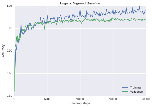
Experiment 1: Variance-adjusted vs. not variance-adjusted REINFORCE
Recall that the REINFORCE estimator estimates the expectation of ∂L∂a as (BSN(a)−sigm(a))(L−c), where c is a constant. The non-variance-adjusted form of REINFORCE uses c=0, whereas the variance-adjusted form uses the variance minimizing result stated above. Naturally we should prefer the least variance, and the experimental results below agree.
It seems that both forms of REINFORCE often break down for learning rates greater than or equal to 0.3 (compare to the learning rate of 1.0 that used in Experiment 0). After a few trials, variance-adjusted REINFORCE appears to be more resistant to such failures.
print("Variance-adjusted:")
res1 = train_classifier(hidden_dims=[100], estimator=StochasticGradientEstimator.REINFORCE, epochs=3,
                       lr=0.3, verbose=True)
print("Not variance-adjusted:")and
res2= train_classifier(hidden_dims=[100], estimator=StochasticGradientEstimator.REINFORCE, epochs=3,
                       lr=0.3, no_var_adj=True, verbose=True)
Variance-adjusted:
Epoch 0 0.1026
Epoch 1 0.4466
Epoch 2 0.511
Epoch 3 0.575
Not variance-adjusted:
Epoch 0 0.0964
Epoch 1 0.0958
Epoch 2 0.0958
Epoch 3 0.0958In terms of performance at lower learning rates, a learning rate of about 0.05 provided the best results. The results show that the variance-adjusted REINFORCE learns faster, but that its non-variance adjusted eventually catches up. This result is consistent with the mathematical result that they are both unbiased estimators. Performance is predictably worse than it was for the plain logistic sigmoid in Experiment 0, although there is almost no generalization gap, consistent with the hypothesis that binary stochastic neurons can act as regularizers.
res1 = train_classifier(hidden_dims=[100], estimator=StochasticGradientEstimator.REINFORCE, epochs=20,
                       lr=0.05, label = "Variance-adjusted")
res2= train_classifier(hidden_dims=[100], estimator=StochasticGradientEstimator.REINFORCE, epochs=20,
                       lr=0.05, no_var_adj=True, label = "Not variance-adjusted")

plot_n(res1 + res2, lower_y=0.6, title="Experiment 1: REINFORCE variance adjustment")
Epoch 20 0.9274
Epoch 20 0.923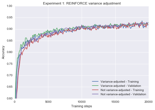
Experiment 2: Pass-through vs. sigmoid-adjusted ST estimation
Recall that one variant of the straight-through estimator uses the identity function as the backpropagated gradient (pass-through), and another variant multiplies that by the gradient of the logistic sigmoid that the neuron calculates (sigmoid-adjusted). In Bengio et al. (2013), it was remarked that, surprisingly, the former performs better. My results below disagree, and by a surprisingly wide margin.
res1 = train_classifier(hidden_dims=[100], estimator=StochasticGradientEstimator.ST, epochs=20,
                       lr=0.1, label = "Pass-through - 0.1")
res2 = train_classifier(hidden_dims=[100], estimator=StochasticGradientEstimator.ST, epochs=20,
                       lr=0.1, slope_annealing_rate = 1.0, label = "Sigmoid-adjusted - 0.1")

res3 = train_classifier(hidden_dims=[100], estimator=StochasticGradientEstimator.ST, epochs=20,
                       lr=0.3, label = "Pass-through - 0.3")
res4 = train_classifier(hidden_dims=[100], estimator=StochasticGradientEstimator.ST, epochs=20,
                       lr=0.3, slope_annealing_rate = 1.0, label = "Sigmoid-adjusted - 0.3")

res5 = train_classifier(hidden_dims=[100], estimator=StochasticGradientEstimator.ST, epochs=20,
                       lr=1.0, label = "Pass-through - 1.0")
res6 = train_classifier(hidden_dims=[100], estimator=StochasticGradientEstimator.ST, epochs=20,
                       lr=1.0, slope_annealing_rate = 1.0, label = "Sigmoid-adjusted - 1.0")

plot_n(res1[1:] + res2[1:] + res3[1:] + res4[1:] + res5[1:] + res6[1:],
       lower_y=0.4, title="Experiment 2: Pass-through vs sigmoid-adjusted ST")
Epoch 20 0.8334
Epoch 20 0.9566
Epoch 20 0.8828
Epoch 20 0.9668
Epoch 20 0.0958
Epoch 20 0.9572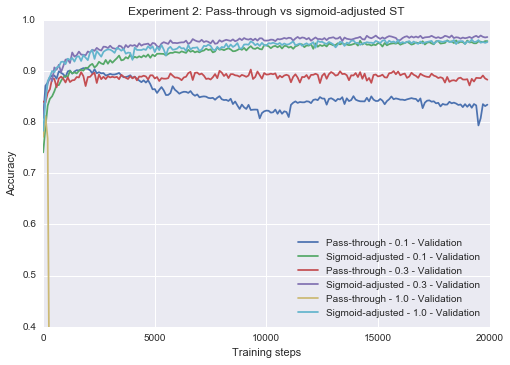
Experiment 3: Pass-through vs. slope-annealed ST estimation
Recall that Chung et al. (2016) improves upon the sigmoid-adjusted variant of the ST estimator by using the slope-annealing trick, which slowly increases the slope of the logistic sigmoid as training progresses. Using the slope-annealing trick with an annealing rate of 1.1 times per epoch (so the slope at epoch 20 is 1.119≈6.1), we’re able to improve upon the sigmoid-adjusted ST estimator, and even beat our non-stochastic, non-binary baseline! Note that the slope annealed neuron used here is not the same as the one used by Chung et al. (2016), who employ a deterministic step function and use a hard sigmoid in place of a sigmoid for the backpropagation.
res1 = train_classifier(hidden_dims=[100], estimator=StochasticGradientEstimator.ST, epochs=20,
                       lr=0.1, slope_annealing_rate = 1.0, label = "Sigmoid-adjusted - 0.1")
res2 = train_classifier(hidden_dims=[100], estimator=StochasticGradientEstimator.ST, epochs=20,
                       lr=0.1, slope_annealing_rate = 1.1, label = "Slope-annealed - 0.1")

res3 = train_classifier(hidden_dims=[100], estimator=StochasticGradientEstimator.ST, epochs=20,
                       lr=0.3, slope_annealing_rate = 1.0, label = "Sigmoid-adjusted - 0.3")
res4 = train_classifier(hidden_dims=[100], estimator=StochasticGradientEstimator.ST, epochs=20,
                       lr=0.3, slope_annealing_rate = 1.1, label = "Slope-annealed - 0.3")

res5 = train_classifier(hidden_dims=[100], estimator=StochasticGradientEstimator.ST, epochs=20,
                       lr=1.0, slope_annealing_rate = 1.0, label = "Sigmoid-adjusted - 1.0")
res6 = train_classifier(hidden_dims=[100], estimator=StochasticGradientEstimator.ST, epochs=20,
                       lr=1.0, slope_annealing_rate = 1.1, label = "Slope-annealed - 1.0")

plot_n(res1[1:] + res2[1:] + res3[1:] + res4[1:] + res5[1:] + res6[1:],
       lower_y=0.6, title="Experiment 3: Sigmoid-adjusted vs slope-annealed ST")
Epoch 20 0.9548
Epoch 20 0.974
Epoch 20 0.9704
Epoch 20 0.9764
Epoch 20 0.9608
Epoch 20 0.9624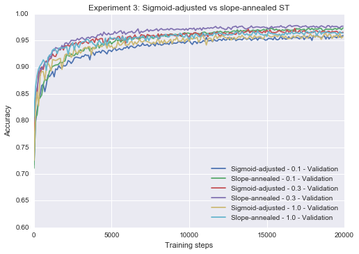
Experiment 4: Variance-adjusted REINFORCE vs slope-annealed ST
We now directly compare the variance-adjusted REINFORCE and slope-annealed ST, both at their best learning rates. In this setting, despite being a biased estimator, the straight-through estimator displays faster learning, less variance, and better overall results than the variance-adjusted REINFORCE estimator.
res1 = train_classifier(hidden_dims=[100], estimator=StochasticGradientEstimator.REINFORCE, epochs=20,
                       lr=0.05, label = "Variance-adjusted REINFORCE")

res2 = train_classifier(hidden_dims=[100], estimator=StochasticGradientEstimator.ST, epochs=20,
                       lr=0.3, slope_annealing_rate = 1.1, label = "Slope-annealed ST")

plot_n(res1[1:] + res2[1:],
       lower_y=0.6, title="Experiment 4: Variance-adjusted REINFORCE vs slope-annealed ST")
Epoch 20 0.926
Epoch 20 0.9782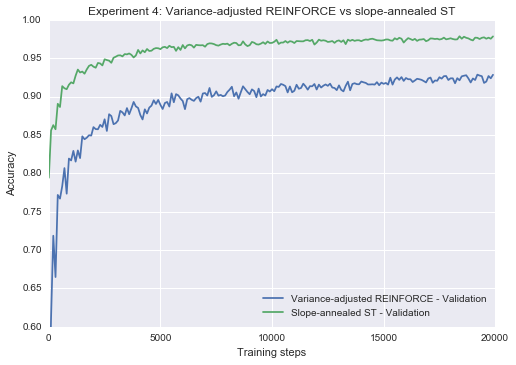
Experiment 5: A look at the deterministic step function, during training and evaluation
Similar to how dropout is not applied at inference when using dropout for training, it makes sense that we might replace the stochastic sigmoid with a deterministic step function at inference when using binary neurons. We might go even further than that, and use deterministic neurons during training, which is the approach taken by Chung et al. (2016). The following three combinations are compared below, using the slope-annealed straight through estimator, without slope annealing:
- stochastic during training, stochastic during test
- stochastic during training, deterministic during test
- deterministic during training, deterministic during test
The results show that deterministic neurons train the fastest, but also display more overfitting and may not achieve the best final results. Stochastic inference and deterministic inference, when combined with stochastic training, are closely comparable. Similar results hold for the REINFORCE estimator.
res1 = train_classifier(hidden_dims=[100], estimator=StochasticGradientEstimator.ST, epochs=20,
                        lr=0.3, slope_annealing_rate = 1.1, label = "Stochastic, Stochastic")
res2 = train_classifier(hidden_dims=[100], estimator=StochasticGradientEstimator.ST, epochs=20,
                        lr=0.3, slope_annealing_rate = 1.1, stochastic_eval=False, label = "Stochastic, Deterministic")
res3 = train_classifier(hidden_dims=[100], estimator=StochasticGradientEstimator.ST, epochs=20,
                        lr=0.3, slope_annealing_rate = 1.1, stochastic_train=False, stochastic_eval=False,
                        label = "Deterministic, Deterministic")

plot_n(res1 + res2 + res3,
       lower_y=0.6, title="Experiment 5: Stochastic vs Deterministic (Slope-annealed ST)")
Epoch 20 0.9776
Epoch 20 0.977
Epoch 20 0.9704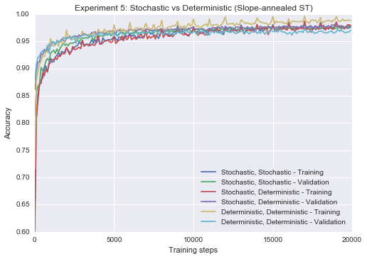
Experiment 6: The effect of depth on REINFORCE and ST estimators
Next, I look at how each estimator interacts with depth. From a theoretical perpective, there is reason to think the straight-through estimator will suffer from depth; as noted by Bengio et al. (2013), it is not even guaranteed to have the same sign as the expected gradient during backpropagation. It turns out that the slope-annealed straight-through estimator is resilient to depth, even at a reasonable learning rate. The REINFORCE estimator, on the other hand, starts to fail as depth is introduced. However, if we lower the learning rate dramatically (25x), we can start to get the deeper networks to train with the REINFORCE estimator.
res1 = train_classifier(hidden_dims=[100], estimator=StochasticGradientEstimator.ST, epochs=20,
                        lr=0.3, slope_annealing_rate=1.1, label = "1 hidden layer")
res2 = train_classifier(hidden_dims=[100, 100], estimator=StochasticGradientEstimator.ST, epochs=20,
                        lr=0.3, slope_annealing_rate=1.1, label = "2 hidden layers")
res3 = train_classifier(hidden_dims=[100, 100, 100], estimator=StochasticGradientEstimator.ST, epochs=20,
                        lr=0.3, slope_annealing_rate=1.1, label = "3 hidden layers")

plot_n(res1[1:] + res2[1:] + res3[1:], title="Experiment 6: The effect of depth (straight-through)")
Epoch 20 0.9774
Epoch 20 0.9738
Epoch 20 0.9728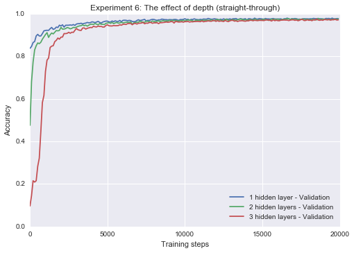
res1 = train_classifier(hidden_dims=[100], estimator=StochasticGradientEstimator.REINFORCE, epochs=20,
                       lr=0.05, label = "1 hidden layer")
res2 = train_classifier(hidden_dims=[100,100], estimator=StochasticGradientEstimator.REINFORCE, epochs=20,
                       lr=0.05, label = "2 hidden layers")
res3 = train_classifier(hidden_dims=[100,100,100], estimator=StochasticGradientEstimator.REINFORCE, epochs=20,
                       lr=0.05, label = "3 hidden layers")

plot_n(res1[1:] + res2[1:] + res3[1:], title="Experiment 6: The effect of depth (REINFORCE)")
Epoch 20 0.9302
Epoch 20 0.8788
Epoch 20 0.2904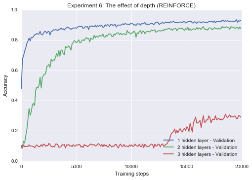
res1 = train_classifier(hidden_dims=[100], epochs=50, non_binary=True,
                       lr=0.002, label = "1 hidden layer")
res2 = train_classifier(hidden_dims=[100,100], epochs=50, non_binary=True,
                       lr=0.002, label = "2 hidden layers")
res3 = train_classifier(hidden_dims=[100,100,100], epochs=50, non_binary=True,
                       lr=0.002, label = "3 hidden layers")

plot_n(res1[1:] + res2[1:] + res3[1:], title="Experiment 6: The effect of depth (REINFORCE) (LR = 0.002)")
Epoch 50 0.931
Epoch 50 0.9294
Epoch 50 0.9096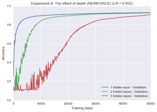
Experiment 7: Using binary stochastic neurons as a regularizer.
I now test the “unpublished result” put forth at the end of Hinton et al.’s Coursera Lecture 9c, which states that we can improve upon the performance of an overfitting multi-layer sigmoid net by turning its neurons binary stochastic neurons with a straight-through estimator.
To test the claim, we will need a dataset that is easier to overfit than MNIST, and so the following experiment uses the MNIST validation set for training (10x smaller than the MNIST training set and therefore much easier to overfit). The hidden layer size is also increased by a factor of 2 to increase overfitting.
We can see below that the stochastic net has a clear advantage in terms of both the generalization gap and training speed, ultimately resulting in a better final fit.
res1 = train_classifier(hidden_dims = [200], epochs=20, train_set=mnist.validation, val_set=mnist.test,
                        lr = 0.03, non_binary = True, label = "Deterministic sigmoid net")

res2 = train_classifier(hidden_dims = [200], epochs=20, stochastic_eval=False, train_set=mnist.validation,
                        val_set=mnist.test, slope_annealing_rate=1.1, estimator=StochasticGradientEstimator.ST,
                        lr = 0.3, label = "Binary stochastic net")

plot_n(res1 + res2, lower_y=0.8, title="Experiment 8: Using binary stochastic neurons as a regularizer")
Epoch 20 0.9276
Epoch 20 0.941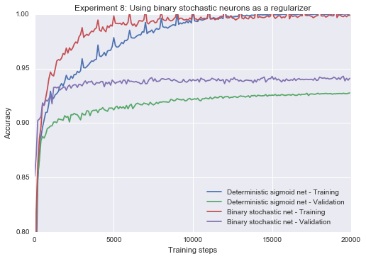
Conclusion
In this post we introduced, implemented and experimented with binary stochastic neurons in Tensorflow. We saw that the biased straight-through estimator generally outperforms the unbiased REINFORCE estimator, and can even outperform a non-stochastic, non-binary sigmoid net. We explored the variants of each estimator, and showed that the slope-annealed straight through estimator is better than other straight through variants, and that it is worth using the variance-adjusted REINFORCE estimator over the not variance-adjusted REINFORCE estimator. Finally, we explored the potential use for binary stochastic neurons as regularizers, and demonstrated that a stochastic binary network trained with the slope-annealed straight through estimator trains faster and generalizes better than an ordinary sigmoid net.
Note: In a previous version of this post, I had instead used dBSN(a)da=BSN(a). This formulation would return the identity if the binary neuron evaluated to 1, and 0 otherwise. I had similarly multiplied the derivatives of the two variants (sigmoid-adjusted and slope-annealed) by a factor of BSN(a). This prior formulation was consistent with my reading of Bengio et al. (2013) and achieved respectable results, but in light of a comment made on this post, and upon review of Hinton’s Coursera lecture where the straight-through estimator is first proposed, I believe the version now reflected in the post, dBSN(a)da=1, is more correct. Although the pass-through variant performs worse with the revised derivative, the sigmoid-adjusted and slope-annealed variants benefit greatly from this change, outperforming both new and old pass-through formulations by a respectable margin.↩