While playing with some applications of binary neurons, I found myself wanting to use explicit activations that go beyond a simple yes/no decision. For example, we might want our neural network to make a choice between several categories (in the form of a one-hot vector) or we might want it to make a choice between ordered categories (e.g., a scale of 1 to 10). It’s rather easy to extend the straight-through estimator to work well on both of these cases, and I thought I would share my work in this post. I share code for implementing ternary and one-hot neurons in Tensorflow, and show that they can learn to solve MNIST.
This is a follow-up post to Binary Stochastic Neurons in Tensorflow, and assumes familiarity with binary neurons and the straight-through estimator discussed therein.
Note Feb. 8, 2017: I haven’t had a chance to read either of these two papers that I came across after writing this post (they look like they are related to the straight-through softmax activation (I think the first offers up an even better estimator… to be decided)):
- Categorical Reparameterization with Gumbel-Softmax
- The Concrete Distribution: A Continuous Relaxation of Discrete Random Variables
I plan to update this post once I get around to reading them.
IPython Notebook: This post is also available as an IPython notebook here.
General n-ary neurons
Whereas the binary neuron outputs 0 or 1, a ternary neuron might output -1, 0, or 1 (or alternatively, 0, 1 or 2). Similarly, we could create an arbitrary n-ary neuron that outputs ordered categories, such as a scale from 1 to 10. Actually, but for the activation function, the code for all of these neurons is the same as the code for the binary neuron: we either round the real output of the activation function to the nearest integer (deterministic), or use its decimal portion to sample either the integer below or the integer above from a bernoulli distribution (stochastic). Note that this means stochastic choices are made only between two adjacent categories, and never across all categories. On the backward pass, we use the straight-through estimator, which means that we replace the gradient of rounding (deterministic) or sampling (stochastic) with the identity. If our activation function is threshholded to [0, 1], this results in a binary neuron, but if it is threshholded to [-1,1], we can output three ordered values.
We might be tempted to use tanh, which is threshholded to [-1, 1], to create ternary neurons. Picking the right activation, however, is a bit trickier than finding a function that has the correct range. The standard tanh is not very good here because its slope near 0 is close to 1, so that a neuron outputting 0 will tend to get pushed away from 0. Instead, we want something that looks like a soft set of stairs (where each step is a sigmoid), so that the neuron can learn to consistently output intermediate values.
With such an activation, a neuron outputting 0 will have a small slope on the backward pass, so that many mistakes (in the same direction) will be required to move it towards 1 or -1.
For the ternary case, the following function works well:
Here is its plot drawn by Wolfram Alpha:
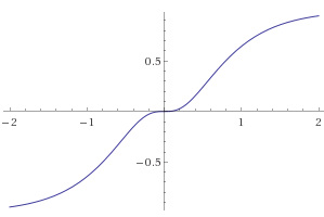
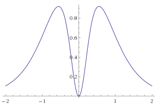
This activation function works well because its slope goes to 0 as it approaches each of the integers in the output range (note that the binary neuron has this property too). Here’s the plot of the derivative for reference:
The above ternary function is implemented below. I’ve been more interested in the one-hot activations, so I haven’t figured out how to make slope annealing work for this ternary neuron, or a general formula for n-ary neurons. If the mathematically-inclined reader would like to leave some ideas in the comments, that would be much appreciated.
One-hot neurons
N-ary neurons are cool, but restrictive. Binary neurons are restricted to yes/no decisions, and ternary+ neurons express the prior that the output categories are linearly ordered. As an example to illustrate this “ordering” point, consider the categories “dislike”, “neutral” and “like”. There is a natural order between these categories (“like” is closer to “neutral” than to “dislike”). Most categories, however, do not have a natural ordering. For example, there is no natural order between Boston, New York and Toronto. To create a neuron that can decided between unordered categories, we would like it to output a one-hot vector like [1, 0, 0] (Boston) or [0, 0, 1] (Toronto). Luckily, the straight through estimator extends nicely to this scenario.
We define a d-dimensional one-hot neuron, as follows. Given an input, , we perform the following steps:
Compute a d-dimensional vector of logits, , where and .
Compute softmax activations, , whose -th component is
where is the -th component of , and is the temperature (used for annealing).
Next, we either sample a one-hot vector according to the distribution defined by (stochastic), or simply use the maximum value of to determine the one-hot output (deterministic). The result is the output of our neuron, . A formal definition of both of these operations is a bit too ugly for this blog post, but this should be fairly straightforward.
Neither sampling from nor using the maximum of have useful (non-zero) gradients. But we can use the straight-through estimator and replace their gradient on the backward pass with the identity. As in the binary case, this leads to a learnable softmax activation.
This definition of one-hot neurons allows for temperature-annealing to be used (note that whereas slope is increased during annealing, temperature is decreased during annealing), which we test below.
Implementation in Tensorflow
Imports and helper functions
import numpy as np, tensorflow as tf, matplotlib.pyplot as plt, seaborn as sns
from tensorflow.examples.tutorials.mnist import input_data
%matplotlib inline
sns.set(color_codes=True)
mnist = input_data.read_data_sets('MNIST_data', one_hot=True)
from tensorflow.python.framework import ops
from collections import Counter

def reset_graph():
    if 'sess' in globals() and sess:
        sess.close()
    tf.reset_default_graph()

def layer_linear(inputs, shape, scope='linear_layer'):
    with tf.variable_scope(scope):
        w = tf.get_variable('w',shape)
        b = tf.get_variable('b',shape[-1:])
    return tf.matmul(inputs,w) + b

def layer_softmax(inputs, shape, scope='softmax_layer'):
    with tf.variable_scope(scope):
        w = tf.get_variable('w',shape)
        b = tf.get_variable('b',shape[-1:])
    return tf.nn.softmax(tf.matmul(inputs,w) + b)

def compute_accuracy(y, pred):
    correct = tf.equal(tf.argmax(y,1), tf.argmax(pred,1))
    return tf.reduce_mean(tf.cast(correct, tf.float32))

def plot_n(data_and_labels, lower_y = 0., title="Learning Curves"):
    fig, ax = plt.subplots()
    for data, label in data_and_labels:
        ax.plot(range(0,len(data)*100,100),data, label=label)
    ax.set_xlabel('Training steps')
    ax.set_ylabel('Accuracy')
    ax.set_ylim([lower_y,1])
    ax.set_title(title)
    ax.legend(loc=4)
    plt.show()
Functions for ternary and n-ary neurons
def st_round(x):
    """Rounds a tensor using the straight through estimator for the gradient."""
    g = tf.get_default_graph()

    with ops.name_scope("StRound") as name:
        with g.gradient_override_map({"Round": "Identity"}):
            return tf.round(x, name=name)
def sample_closest_ints(x):
"""If x is a float, then samples floor(x) with probability x - floor(x), and ceil(x) with
probability ceil(x) - x, using the straight through estimator for the gradient.
E.g.,:
if x is 0.6, sample_closest_ints(x) will be 1 with probability 0.6, and 0 otherwise,
and the gradient will be pass-through (identity).
"""
with ops.name_scope("SampleClosestInts") as name:
with tf.get_default_graph().gradient_override_map({"Ceil": "Identity","Sub": "SampleClosestInts"}):
return tf.ceil(x - tf.random_uniform(tf.shape(x)), name=name)
@ops.RegisterGradient("SampleClosestInts")
def sample_closest_ints_grad(op, grad):
return [grad, tf.zeros(tf.shape(op.inputs[1]))]def binary_activation(x, slope_tensor):
return tf.cond(tf.equal(1., slope_tensor),
lambda: tf.sigmoid(x),
lambda: tf.sigmoid(slope_tensor * x))
def ternary_activation(x, slope_tensor = None, alpha = 1):
"""
Does not support slope annealing (slope_tensor is ignored)
Wolfram Alpha plot:
https://www.wolframalpha.com/input/?i=plot+(1.5*tanh(x)+%2B+0.5(tanh(-(3-1e-2)*x))),+x%3D+-2+to+2
"""
return 1.5*tf.tanh(alpha*x) + 0.5*(tf.tanh(-(3/alpha)*x))def n_ary_activation(x, activation=binary_activation, slope_tensor=None, stochastic_tensor=None):
"""
n-ary activation for creating binary and ternary neurons (and n-ary neurons, if you can
create the right activation function). Given a tensor and an activation, it applies the
activation to the tensor, and then either samples the results (if stochastic tensor is
true), or rounds the results (if stochastic_tensor is false) to the closest integer
values. The default activation is a sigmoid (when slope_tensor = 1), which results in a
binary neuron, as in http://r2rt.com/binary-stochastic-neurons-in-tensorflow.html.
Uses the straight through estimator during backprop. See https://arxiv.org/abs/1308.3432.
Arguments:
* x: the pre-activation / logit tensor
* activation: sigmoid, hard sigmoid, or n-ary activation
* slope_tensor: slope adjusts the slope of the activation function, for purposes of the
Slope Annealing Trick (see http://arxiv.org/abs/1609.01704)
* stochastic_tensor: whether to sample the closest integer, or round to it.
"""
if slope_tensor is None:
slope_tensor = tf.constant(1.0)
if stochastic_tensor is None:
stochastic_tensor = tf.constant(True)
p = activation(x, slope_tensor)
return tf.cond(stochastic_tensor,
lambda: sample_closest_ints(p),
lambda: st_round(p))Functions to make a layer of one-hot neurons
def st_sampled_softmax(logits):
    """Takes logits and samples a one-hot vector according to them, using the straight
    through estimator on the backward pass."""
    with ops.name_scope("STSampledSoftmax") as name:
        probs = tf.nn.softmax(logits)
        onehot_dims = logits.get_shape().as_list()[1]
        res = tf.one_hot(tf.squeeze(tf.multinomial(logits, 1), 1), onehot_dims, 1.0, 0.0)
        with tf.get_default_graph().gradient_override_map({'Ceil': 'Identity', 'Mul': 'STMul'}):
            return tf.ceil(res*probs)

def st_hardmax_softmax(logits):
    """Takes logits and creates a one-hot vector with a 1 in the position of the maximum
    logit, using the straight through estimator on the backward pass."""
    with ops.name_scope("STHardmaxSoftmax") as name:
        probs = tf.nn.softmax(logits)
        onehot_dims = logits.get_shape().as_list()[1]
        res = tf.one_hot(tf.argmax(probs, 1), onehot_dims, 1.0, 0.0)
        with tf.get_default_graph().gradient_override_map({'Ceil': 'Identity', 'Mul': 'STMul'}):
            return tf.ceil(res*probs)

@ops.RegisterGradient("STMul")
def st_mul(op, grad):
    """Straight-through replacement for Mul gradient (does not support broadcasting)."""
    return [grad, grad]

def layer_hard_softmax(x, shape, onehot_dims, temperature_tensor=None, stochastic_tensor=None,
                       scope='hard_softmax_layer'):
    """
    Creates a layer of one-hot neurons. Note that the neurons are flattened before returning,
    so that the shape of the layer needs to be a multiple of the dimension of the one-hot outputs.

    Arguments:
    * x: the layer inputs / previous layer
    * shape: the tuple of [size_previous, layer_size]. Layer_size must be a multiple of onehot_dims,
        since each neuron's output is flattened (i.e., the number of neurons will only be
        layer_size / onehot_dims)
    * onehot_dims: the size of each neuron's output
    * temperature_tensor: the temperature for the softmax
    * stochastic_tensor: whether the one hot outputs are sampled from the softmax distribution
        (stochastic - recommended for training), or chosen according to its maximal element
        (deterministic - recommended for inference)
    """
    assert(len(shape) == 2)
    assert(shape[1] % onehot_dims == 0)
    if temperature_tensor is None:
        temperature_tensor = tf.constant(1.)
    if stochastic_tensor is None:
        stochastic_tensor = tf.constant(True)

    with tf.variable_scope(scope):
        w = tf.get_variable('w',shape)
        b = tf.get_variable('b',shape[-1:])
    logits = tf.reshape((tf.matmul(x, w) + b) / temperature_tensor,
                        [-1, onehot_dims])

    return tf.cond(stochastic_tensor,
                lambda: tf.reshape(st_sampled_softmax(logits), [-1, shape[1]]),
                lambda: tf.reshape(st_hardmax_softmax(logits), [-1, shape[1]]))
Function to build graph for MNIST classifier
def build_classifier(hidden_dims=[100],
                     lr = 0.5,
                     activation=binary_activation,
                     onehot_dims = 0):
    reset_graph()

    """Placeholders"""
    x = tf.placeholder(tf.float32, [None, 784], name='x_placeholder')
    y = tf.placeholder(tf.float32, [None, 10], name='y_placeholder')
    stochastic_tensor = tf.constant(True)
    slope_tensor = tf.constant(1.0)
    temperature_tensor = 1 / slope_tensor

    layers = {0: x}
    num_hidden_layers = len(hidden_dims)
    dims = [784] + hidden_dims

    for i in range(1, num_hidden_layers+1):
        with tf.variable_scope("layer_" + str(i)):
            if onehot_dims:
                layers[i] = layer_hard_softmax(layers[i-1],
                                              dims[i-1:i+1],
                                              onehot_dims,
                                              temperature_tensor,
                                              stochastic_tensor)
            else:
                pre_activations = layer_linear(layers[i-1], dims[i-1:i+1], scope='layer_' + str(i))
                if activation is tf.tanh or activation is tf.sigmoid:
                    layers[i] = activation(pre_activations)
                else:
                    layers[i] = n_ary_activation(pre_activations,
                                               activation,
                                               slope_tensor,
                                               stochastic_tensor)

    final_hidden_layer = layers[num_hidden_layers]
    preds = layer_softmax(final_hidden_layer, [dims[-1], 10])
    loss = -tf.reduce_mean(y * tf.log(preds), reduction_indices=1)
    ts = tf.train.GradientDescentOptimizer(lr).minimize(loss)

    accuracy = compute_accuracy(y, preds)

    return dict(
        x=x,
        y=y,
        stochastic=stochastic_tensor,
        slope=slope_tensor,
        final_hidden_layer = final_hidden_layer,
        loss=loss,
        ts=ts,
        accuracy=accuracy,
        init_op=tf.global_variables_initializer()
    )
Function to train the classifier
def train_classifier(\
        hidden_dims=[100,100],
        activation=binary_activation,
        onehot_dims = 0,
        stochastic_train=True,
        stochastic_eval=True,
        slope_annealing_rate=None,
        epochs=20,
        lr=0.5,
        verbose=True,
        label=None):
    g = build_classifier(hidden_dims=hidden_dims, lr=lr,
        activation=activation, onehot_dims=onehot_dims)

    with tf.Session() as sess:
        sess.run(g['init_op'])
        slope = 1
        res_tr, res_val, sample_layers = [], [], []
        for epoch in range(epochs):
            feed_dict={g['x']: mnist.validation.images,
                       g['y']: mnist.validation.labels,
                       g['stochastic']: stochastic_eval,
                       g['slope']: slope}
            acc, final_hidden = sess.run([g['accuracy'], g['final_hidden_layer']],
                                            feed_dict=feed_dict)
            sample_layers.append(final_hidden)
            if verbose:
                print("Epoch", epoch, acc)
            else:
                print('.', end='')

            accuracy = 0
            for i in range(1,1001):
                x, y = mnist.train.next_batch(50)
                feed_dict={g['x']: x, g['y']: y, g['stochastic']: stochastic_train}
                acc, _ = sess.run([g['accuracy'],g['ts']], feed_dict=feed_dict)
                accuracy += acc
                if i % 100 == 0 and i > 0:
                    res_tr.append(accuracy/100)
                    accuracy = 0
                    feed_dict={g['x']: mnist.validation.images,
                               g['y']: mnist.validation.labels,
                               g['stochastic']: stochastic_eval,
                               g['slope']: slope}
                    res_val.append(sess.run(g['accuracy'], feed_dict=feed_dict))

            if slope_annealing_rate is not None:
                slope = slope*slope_annealing_rate
                if verbose:
                    print("Annealed slope:", slope, "| Annealed temperature:", 1/ slope)

        feed_dict={g['x']: mnist.validation.images, g['y']: mnist.validation.labels,
                   g['stochastic']: stochastic_eval, g['slope']: slope}
        print("\nFinal epoch, epoch", epoch+1, ":", sess.run(g['accuracy'], feed_dict=feed_dict))

        if label is not None:
            return (res_tr, label + " - Training"), (res_val, label + " - Validation")
        else:
            return [(res_tr, "Training"), (res_val, "Validation")], sample_layers
Experiments
Let us now demonstrate that the above neurons train on MNIST, and can achieve reasonably good results. I’m not hunting for hyperparameters here, so the below may not be optimal. All training is done over 20 epochs with a learning rate of 0.1.
Tanh baseline (real-valued activations)
res, _ = train_classifier(hidden_dims=[100], activation=tf.tanh, epochs=20, lr=0.1, verbose=False)
plot_n(res, lower_y=0.8, title="Tanh Baseline")
....................
Final epoch, epoch 20 : 0.9772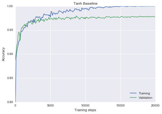
Binary neurons with slope annealing baseline
More results on binary neurons available in my prior post.
res, _ = train_classifier(hidden_dims=[100], activation=binary_activation, epochs=20, lr=0.1,
                                      slope_annealing_rate=1.1, stochastic_eval=False, verbose=False)
plot_n(res, lower_y=0.8, title="Binary Stochastic w/ Slope Annealing Baseline")
....................
Final epoch, epoch 20 : 0.9732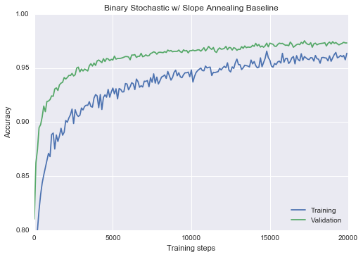
Ternary neurons
As noted above, I didn’t spend the time to figure out a good way to slope-anneal the ternary activation, so the below is not slope-annealed.
The interesting thing to note is that these neurons are more expressive than the binary neurons, and so they not only get closer to the tanh baseline, but they also offer less regularization / overfit more quickly.
res, sample_layers = train_classifier(hidden_dims=[100], activation=ternary_activation, epochs=20, lr=0.1,
                                      stochastic_eval=False, verbose=False)
plot_n(res, lower_y=0.8, title="Ternary Stochastic")
....................
Final epoch, epoch 20 : 0.9764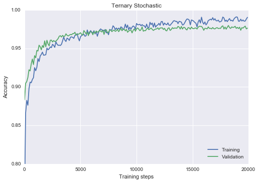
If you’re curious as to the distribution of outputs, here it is:
c = Counter(np.reshape(sample_layers[-1], [-1]))
g = sns.barplot(x = list(c.keys()), y = list(c.values()))
sns.plt.title('Distribution of ternary outputs on MNIST')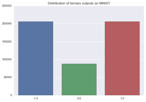
One-hot neurons
First, let’s take a look at what the layer activations look like, in case my description above wasn’t super clear. We’ll pull out the last layer of a network that uses 100 5-dimensional one-hot neurons, and then “unflatten” it into shape [100, 5].
res, sample_layers = train_classifier(hidden_dims=[500], onehot_dims=5, epochs=20, lr=0.1,
                                      stochastic_eval=False, verbose=False)
....................
Final epoch, epoch 20 : 0.9794Here is what the activations of the first 10 neurons of the first sample in the validation set look like. As discussed, each neuron outputs a 5D one-hot vector:
np.reshape(sample_layers[0][0], [100, 5])[:10]array([[ 0., 0., 0., 0., 1.],
[ 0., 1., 0., 0., 0.],
[ 0., 0., 0., 1., 0.],
[ 0., 0., 1., 0., 0.],
[ 1., 0., 0., 0., 0.],
[ 0., 0., 1., 0., 0.],
[ 0., 0., 1., 0., 0.],
[ 0., 1., 0., 0., 0.],
[ 0., 0., 0., 1., 0.],
[ 0., 1., 0., 0., 0.]], dtype=float32)One-hot neurons: temperature annealing
Now, let’s test some 5D neurons to see if temperature annealing does anything. Looks like not really:
_, res1 = train_classifier(hidden_dims=[500], onehot_dims=5, epochs=20, lr=0.1,
                                      stochastic_eval=False,
                                      label= "No temperature annealing", verbose=False)
_, res2 = train_classifier(hidden_dims=[500], onehot_dims=5, epochs=20, lr=0.1,
                                      slope_annealing_rate=1.2, stochastic_eval=False,
                                      label= "Annealing rate 1.2", verbose=False)
_, res3 = train_classifier(hidden_dims=[500], onehot_dims=5, epochs=20, lr=0.1,
                                      slope_annealing_rate=1.5, stochastic_eval=False,
                                      label= "Annealing rate 1.5", verbose=False)
plot_n([res1] + [res2] + [res3], lower_y=0.8, title="5D one-hot neurons, temperature annealing (validation)")
....................
Final epoch, epoch 20 : 0.981
....................
Final epoch, epoch 20 : 0.9796
....................
Final epoch, epoch 20 : 0.9798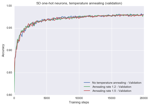
One-hot neurons: number of dimensions
We can also easily change with the number of dimensions of each neuron. I keep the layer size constant in terms of the number of neurons, but make them progressively more expressive and see what happens (because layers are flattened, it appears that the layer size is growing, but the number of neurons stays the same). Looks like not much happens, but maybe this has to do with the simplicity of the dataset. Query whether more expressive one-hot neurons would make a difference on a harder dataset. Note: I plotted the training curves locally, and they show the same result (I would have thought higher dimensional neurons would fit the training data better, but apparently not – perhaps due to stochasticity).
_, res1 = train_classifier(hidden_dims=[300], onehot_dims=3, epochs=20, lr=0.1, stochastic_eval=False,
                                      label= "3 dimensions", verbose=False)
_, res2 = train_classifier(hidden_dims=[500], onehot_dims=5, epochs=20, lr=0.1, stochastic_eval=False,
                                      label= "5 dimensions", verbose=False)
_, res3 = train_classifier(hidden_dims=[700], onehot_dims=7, epochs=20, lr=0.1, stochastic_eval=False,
                                       label= "7 dimensions", verbose=False)
_, res4 = train_classifier(hidden_dims=[1000], onehot_dims=10, epochs=20, lr=0.1, stochastic_eval=False,
                                       label= "10 dimensions", verbose=False)
plot_n([res1] + [res2] + [res3] + [res4], lower_y=0.8, title="N-dimensional one-hot neurons")
....................
Final epoch, epoch 20 : 0.9772
....................
Final epoch, epoch 20 : 0.98
....................
Final epoch, epoch 20 : 0.981
....................
Final epoch, epoch 20 : 0.9754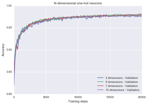
Conclusion
That’s it for now! In this post we saw how we can use the straight-through estimator to create expressive trainable explicit neurons. In particular, we coded up neurons that can represent more than 2 ordered categories (the ternary, or general n-ary neuron), and also neurons that can represent 3 or more unordered categories (the one-hot neuron). Moreover, we showed that they are all competitive with a real-valued tanh baseline on MNIST, and that they provide strong built-in regularization.
I discuss any applications in this post, but I’m hoping to show you something really cool using one-hot neurons in the next one.